Conditional Formatting allows you to format a cell or a range of cells based on the data of another cell. This helps you to highlight important data and increases visibility. However, this is a tricky process that needs clarification to process smoothly.
In this article, we will review various examples that will help you easily apply conditional formatting in your Google Sheets.
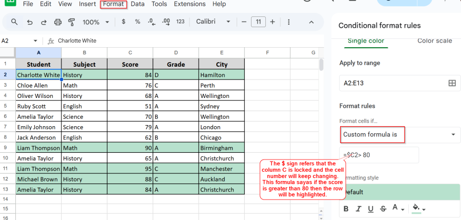
➤ Go to Format > Conditional Formatting > Custom formula to apply a custom conditional formatting. Then enter the formula of your choice.
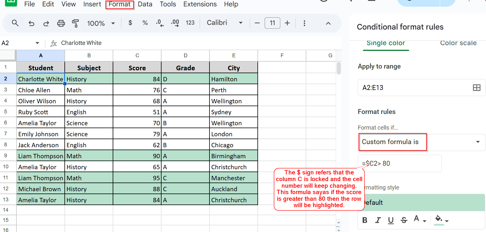
➤ To identify students with scores over 80, you need to use the =$C2> 80 formula. We have used the $ sign to lock down the C column.
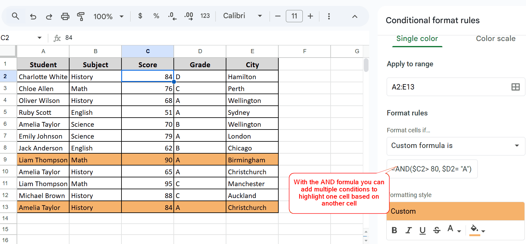
➤ You also apply two conditions at a time. When both conditions are met, the cells are highlighted. To apply two conditions simultaneously, just use the AND formula.
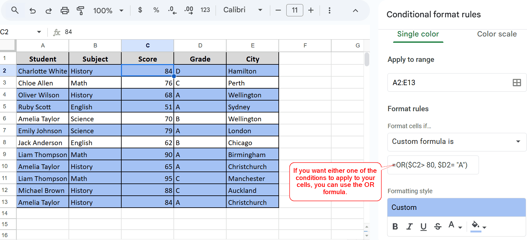
➤ If you want to apply either of the two conditions and highlight the cells, use the OR formula.
Applying One Conditional Formatting Rule
Highlighting cells based on one conditional formatting is pretty straightforward. Let’s say we want to highlight the student rows who have a score over 80. Here’s how you can do it:
Steps:
➤ Highlight all the cells you want the condition to apply to. I want to use conditional formatting on all my data, so I have selected A2 to E13.
➤ Now, open the conditional formatting function from Format > Conditional Formatting.
➤ Select ‘Custom formula is’ from the ‘Format rules’ dropdown.
➤ Apply this formula:
=$C2> 80
➤ Choose your preferred Formatting style and hit Done. That’s it! Now you have formatted the cells based on the Score cell.
Note:
When you are applying the formula, you must start with an active cell after the ‘=’ sign. When you have selected your range, you will notice one active cell.
Applying Two Conditional Formatting Rules at a Time
Now that you know how to apply one conditional formatting based on another cell, adding two or even three conditional formatting is as easy as a breeze. Now, we will be using two conditional formats for our data.
For example, we want to find students who have scores over 80 and an ‘A’ grade overall.
Steps:
➤ Just like the previous example, select all the data and open conditional formatting.
➤ After you have selected ‘Custom formula is’, apply this formula:
=AND($C2> 80, $D2= “A”)
This AND represents a string, where both of these conditions are true.
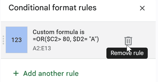
➤ You can also apply two conditions, but highlight rows if either one of those conditions is true. For that, you just have to replace the AND with an OR formula like this:
=OR($C2> 80, $D2= “A”)
Frequently Asked Questions
How to Remove Conditional Formatting in Google Sheets?
It’s easy to remove/delete conditional formatting. Simply click the cell where you have applied conditional formatting, and a sidebar will open on the right corner. As you hover your cursor, a Delete button will appear. Click on the button, and you are all done.
How Do You Format Cells Based on Another Sheet?
Open the Conditional Formatting from the Format section. Choose ‘Custom formula is’, then apply this formula: =INDIRECT(“Sheet2!C1”).
How Does Conditional Formatting Work in the Case of Overlap?
Google Sheets prioritizes the ascending order. It would show the highlighted color in the order in which you have applied your conditions. If you want to change the order, you can simply drag and change it.
Concluding Words
Conditional formatting based on another cell is easy when you know the breakdown of the formula. We have shown you three examples and a complete breakdown of each formula.
We have used the custom formulas only to give you a complete insight. However, a few built-in formulas can be your friend, too. Please let us know in the comments if you have any queries or confusion. We would love to hear your thoughts on our explanation!