When working on a spreadsheet, we often need to analyze our data in numerous ways. Sometimes, we might want to check every other row to find a pattern or sort some data. Removing every other row for a quick view sounds easy, but it can be hard sometimes. In this article, we will show you four ways on how to delete every other row in google sheets.
Steps to delete every other row in google sheets:
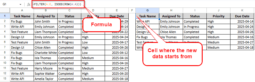
➤ Select the cell from where you want to see the newly sorted data without every other row
➤ Enter this formula in the formula bar:
=FILTER(A:E, ISODD(ROW(A:A)))
➤ Replace A:E with your first and last column, and A:A with the first column name.
➤ Replace ISODD to ISEVEN if you want to delete odd rows, or keep it the same to delete even rows.
➤ Press “Enter” to get the new data without every other row

There are many ways you can delete every other row from your google sheet. In this article, we will show you step by step how to do it. No matter whether you are a beginner or an expert, you can learn something new from this article.
Using Formula with FILTER Function
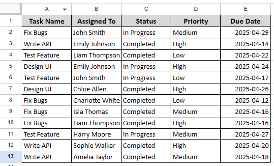
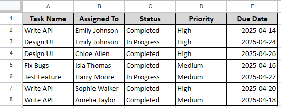
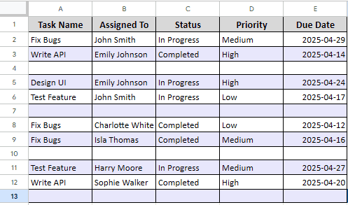
Here in the sample dataset, we have some project tasks for a coding team. The team members use this list to keep track of deadlines and let others know about their progress. For project management, it might be crucial to know about every other tasks. Fortunately, that can be easily done using google sheets. Check the simple methods shown below.
The simplest method to do this job is to use a formula. Follow these steps to apply this method:
➤ Select a new cell from where the new table without every other row will be created.
➤ Enter this formula:
=FILTER(!A:E, ISODD(ROW(A:A)))
➤ If you want to keep the ODD rows, you must change ISODD to ISEVEN. That function keeps the row it is named after, so you must use the opposite.
➤ Press Enter.
➤ Delete the old sheet if you want by right-clicking Sheet1 and clicking “Delete”.
Using a Helper Column
If you don’t want new data and instead just want to see every other row, this is the method you should use. Follow these steps:
➤ Go to the first column on the right of your dataset. This will be your helper column.
➤ On the second cell of that column (because the first row is for the table header), write this formula:
=ISEVEN(ROW())
➤ Press Enter, then drag the fill handle to the bottom of the sheet (as much data as you have)
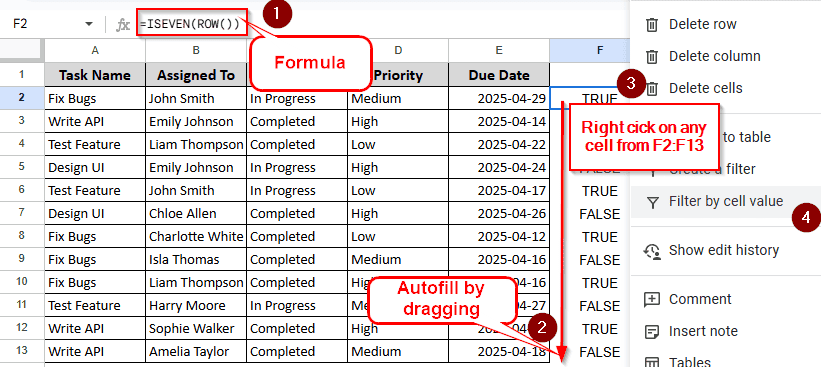
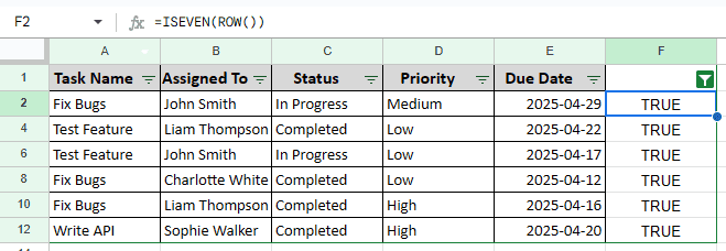
➤ Now, to hide the odd rows, right-click on any “TRUE” cell, and click “Filter by cell value”. Click on the “FALSE” cell and do the same for hiding the even rows.
Using AppScript Code
Now we are officially entering the hard mode. Google sheets allow you to use your custom code to do stuff. We are going to use some coding to achieve our results. Follow these simple steps to delete every other row in google sheets.
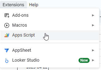
➤ Go to Extensions > Apps Script. A new tab will open.
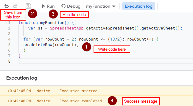
➤ The new tab will have a code editor that will allow you to use your own code. Write this code in the window:
function myFunction() {
var ss = SpreadsheetApp.getActiveSpreadsheet().getActiveSheet();
for (var rowCount = 2; rowCount <= (13/2); rowCount++) {
ss.deleteRow(rowCount);
}
}
➤ Set rowCount in the third line to 1 if you want to delete odd rows. In the section where it says 13/2, you need to replace 13 with the amount of rows you have.
➤ Save and run the script. It might ask for some permissions. After granting them, you will see the message “Execution completed” in the execution logs.
➤ Go back to your sheet to see the results.
Deleting Every Nth Row
So far, we have tried deleting every even or odd row. But what if there is a scenario when you need to delete, say, every 3rd or 4th, or 6th row? This is how you do it.
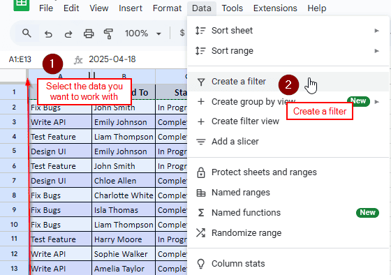
➤ Select all your data, including the heading row.
➤ Go to Data > Select the option Create a filter from the menu at the top.
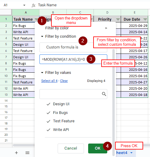
➤ Now you will see a dropdown marker at the top row. Click on it to open the dropdown menu.
➤ Open “Filter by condition”. There should be a scroll-down menu with it that says “None”. You have to select “Custom Formula is” and write this formula:
=MOD(ROW(A1:A16),3)=0
➤ Change A1:A16 to your data range. The 3 in this formula is for every 3rd row. You can change it to 4, 5, or anything else you want. Then click OK.
➤ Now you will see every Nth row in the table. Delete those values.
➤ Go to Data > Remove filter. Your work is done.
Frequently Asked Questions
How do I select every other row in Google Sheets?
From the very left, select the first row (or second if that’s what you prefer). Then hold the Ctrl key on your Windows/Linux keyboard, or the Cmd key if you are on Mac. Then click on every other row to select them.
How do I extract every other row in Excel?
Use this formula:
=FILTER(A:E, MOD(ROW(A:E), 2) = 0)
Here A:E is the range of rows, modify it according to the range of data your dataset has.
How do I color every other row in Google Sheets?
You need to select your dataset first. Then go to the topbar. From the “Format” menu, select “Alternating colors”.
How do I select all rows in Google Sheets?
This is the same as the default select all shortcut on Windows. Just press “Ctrl+A” to select all the rows in a google sheet.
How do I delete duplicate rows in Google Sheets?
First, select the rows you want to delete duplicate rows from. Then go to “Data>Data cleanup>Remove duplicates” from the menu in the top bar. Select your variables and remove the duplicate rows.
Wrapping Up
In this article, we learned four methods on how to delete every other row in google sheets. Hope that you can use those methods for removing rows from your dataset as well. Feel free to use the practice file, and leave a comment with your suggestions.