In many real-world cases, you might not want people to type anything into a spreadsheet freely. You want to limit what users can enter based on conditions, and often, those conditions depend on another cell’s value.
In this article, you’ll learn how to set up data validation rules that change based on another cell, apply them across multiple rows, and use Apps Script to copy these validations without breaking the logic.
Steps to apply conditional data validation using a reference cell on the same row:
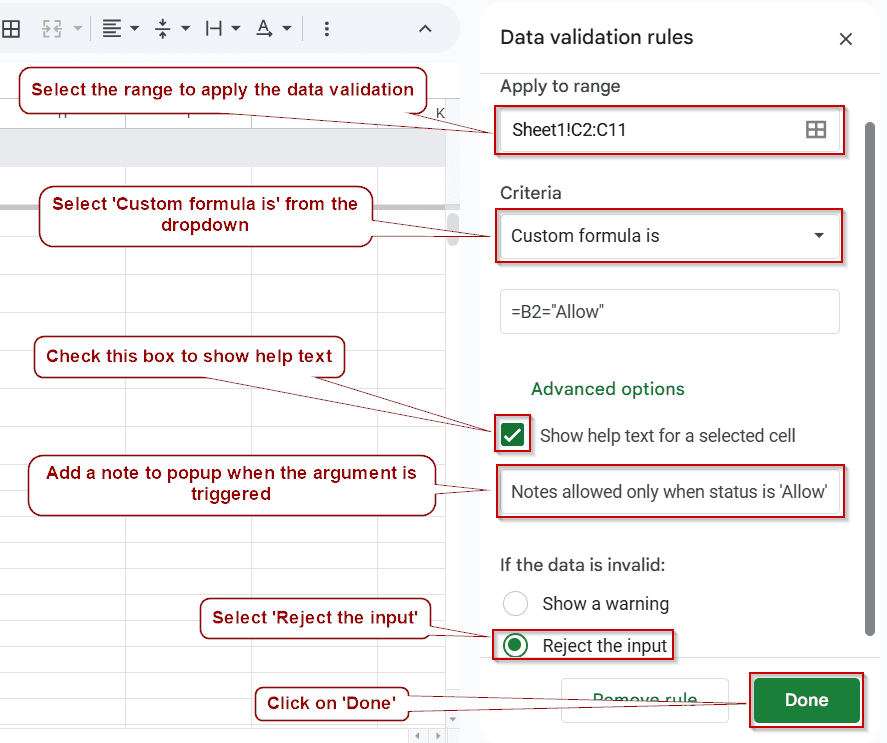
➤ Select the range C2:C11 which contains the Notes column you want to validate.
➤ Go to Data >> Data validation and under Criteria, choose Custom formula is.
➤ Enter the formula =B2=”Allow” to make each Notes cell depend on its corresponding Status cell.
➤ Enable “Reject input” and optionally add help text such as “Notes allowed only when status is ‘Allow’“.
➤ Click Done to apply the validation. Each Notes cell will now allow input only if the Status in the same row is “Allow“.
Use a Fixed Cell to Control Entry Globally
This method is useful when you want all entries in a column to depend on a single controlling cell.
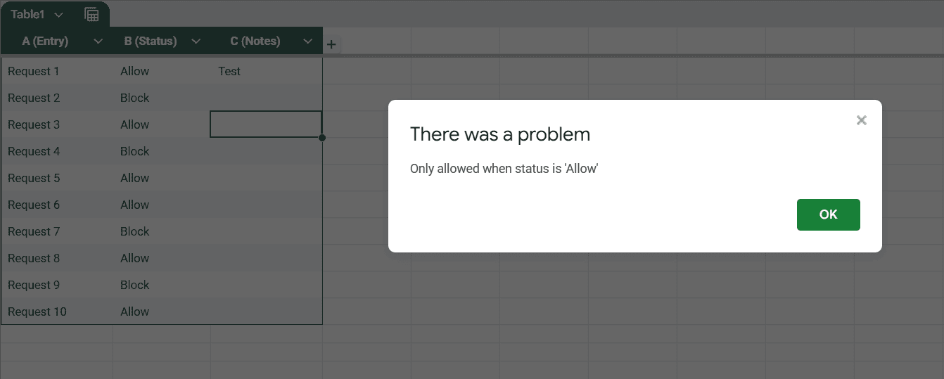
We’re using an approval tracker that lists Requests in column A, their Status in column B, and a Notes column in column C.
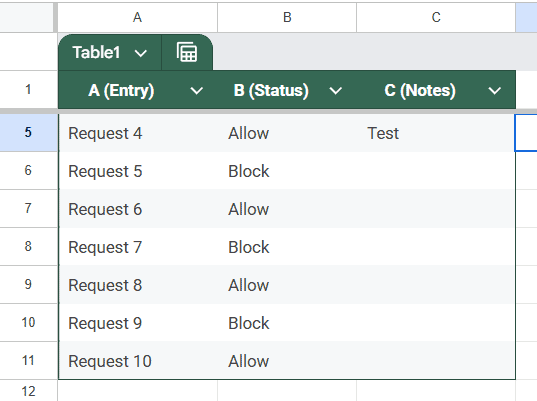
In this case, we’ll apply data validation to the Notes column so that users can only type in it when cell B2 contains the word “Allow.” This setup is helpful when you want a central toggle to enable or block inputs across multiple rows. Make sure your dataset has a clearly defined controlling cell before applying the rule.
Steps:
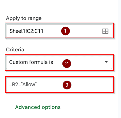
➤ Select range C2:C11 in the Notes column.
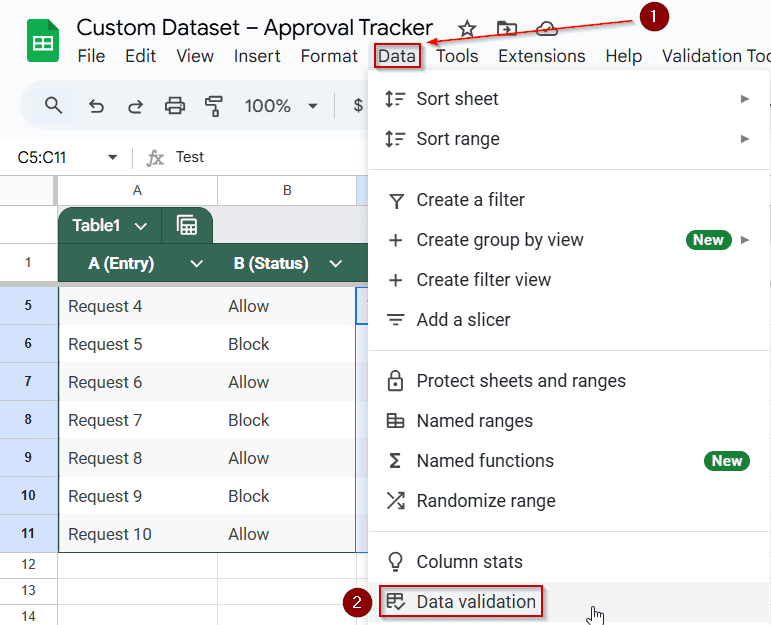
➤ Go to Data >> Data validation.
➤ Choose Custom formula under Criteria.
➤ Enter this formula:
=$B$2=”Allow”
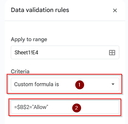
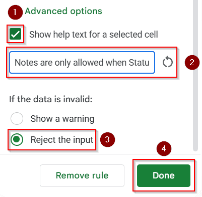
➤ Set the validation to Reject input.
➤ Optionally, add a help text like: “Notes are only allowed when Status in B2 is ‘Allow’“
 ➤ Click Done.
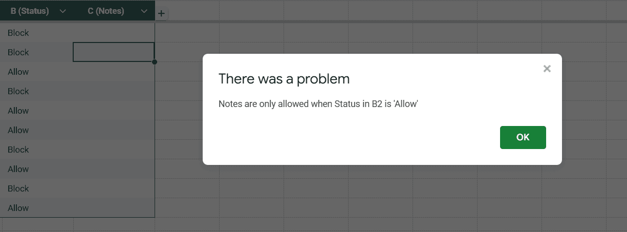
Now, all Notes cells will only accept input when B2 specifically says “Allow”.
Validate Notes Based on the Status in the Same Row
This is the most practical method for forms or trackers where each row is independent.
Steps:
➤ Select C2:C11
➤ Go to Data >> Data validation

➤ Under Criteria, select Custom formula is
➤ Enter this formula:
=B2=”Allow”
➤ Enable Reject input
➤ Add help text if needed
➤ Click Done
Now:
➤ If row 2 has Status = “Allow“, the user can type in C2
➤ If row 3 has Status = “Block“, C3 is locked
➤ And so on…
This keeps the validation row-aware.
Use Apps Script to Copy Row-Based Validation Down
By default, if you drag a validated cell down, the formula reference doesn’t update. To fix this, use a custom script that copies a formula-based validation across rows and adjusts it.
Steps:
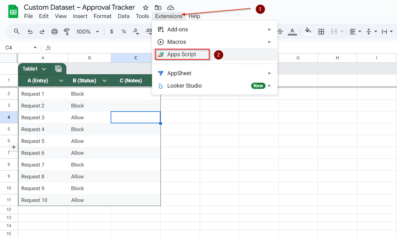
➤ Go to Extensions >> Apps Script
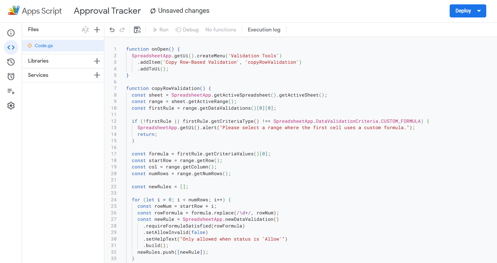
➤ Delete any existing code and paste this custom script:
function onOpen() {
SpreadsheetApp.getUi().createMenu('Validation Tools')
.addItem('Copy Row-Based Validation', 'copyRowValidation')
.addToUi();
}
function copyRowValidation() {
const sheet = SpreadsheetApp.getActiveSpreadsheet().getActiveSheet();
const range = sheet.getActiveRange();
const firstRule = range.getDataValidations()[0][0];
if (!firstRule || firstRule.getCriteriaType() !== SpreadsheetApp.DataValidationCriteria.CUSTOM_FORMULA) {
SpreadsheetApp.getUi().alert("Please select a range where the first cell uses a custom formula.");
return;
}
const formula = firstRule.getCriteriaValues()[0];
const startRow = range.getRow();
const col = range.getColumn();
const numRows = range.getNumRows();
const newRules = [];
for (let i = 0; i < numRows; i++) {
const rowNum = startRow + i;
const rowFormula = formula.replace(/\d+/, rowNum);
const newRule = SpreadsheetApp.newDataValidation()
.requireFormulaSatisfied(rowFormula)
.setAllowInvalid(false)
.setHelpText("Only allowed when status is 'Allow'")
.build();
newRules.push([newRule]);
}
sheet.getRange(startRow, col, numRows).setDataValidations(newRules);
}
➤ Save the script and refresh your sheet.
➤ A new menu called Validation Tools will appear.
➤ Select the cell where you already have a working formula like =B2=”Yes” in validation.
➤ Select the full column (e.g., C2:C11)
➤ From the Validation Tools menu, click Copy Relative Validation
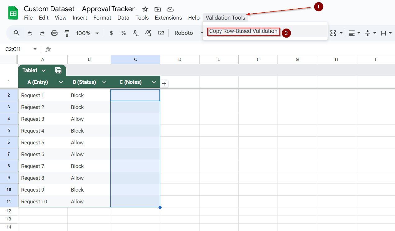
Now, the formula will adjust row by row: C2 will check B2, C3 will check B3, and so on. No manual setup is needed.
Frequently Asked Questions
How do I make a cell in Google Sheets only allow input if another cell has a specific value?
Use Data >> Data validation, choose Custom formula is, and enter a formula like =B2=”Allow” to allow input conditionally.
Can I apply data validation across multiple rows using different reference cells?
Yes. For row-specific rules, use a formula like =B2=”Allow” with relative referencing and apply it to the full range (e.g., C2:C100).
Why doesn’t my validation formula update when I copy it down?
Google Sheets does not auto-adjust data validation formulas when dragged. Use an Apps Script to replicate row-relative validations properly.
Can I restrict input based on a dropdown value in another cell?
Yes. If your dropdown cell is, for example, B2, use =B2=”Approved” as the custom validation formula for the target cell.
How do I show a message when invalid data is entered?
In the data validation menu, enable Show validation help text and set a custom message. It appears when someone enters invalid data.
Wrapping Up
Data validation based on another cell in Google Sheets allows you to create smarter, rule-driven spreadsheets. Whether locking fields until a specific condition is met or creating approval logic, these methods give you full control over input behavior. Choose between basic formulas or advanced scripting depending on your workflow and team needs.