Drop-down lists in Google Sheets are great for organizing data, but you can make them even more powerful by using them to update other cell values automatically. Whether you’re building a form, a tracker, or a dynamic report, this feature lets you set up automatic responses based on what someone selects from a drop-down list.
In this article, you’ll learn several methods for updating cell values based on drop-down selections. We will use formulas like IF, VLOOKUP, and even Google Apps Script for more advanced automation.
Steps to auto-fill the Level column based on the Department drop-down selection:
➤ Select the range B2:B11, where the department dropdown will be applied.
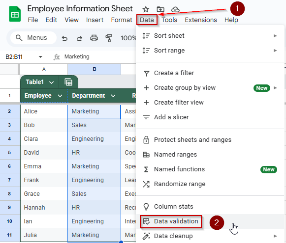
➤ Go to the top menu and click Data >> Data validation.
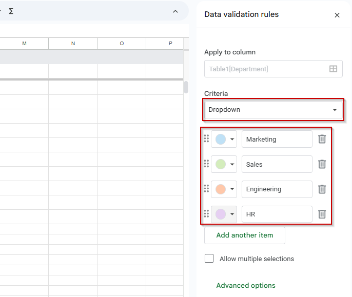
➤ Under Criteria, choose Drop-down. If Google Sheets doesn’t auto-detect values, manually enter: Marketing, Sales, Engineering, HR.
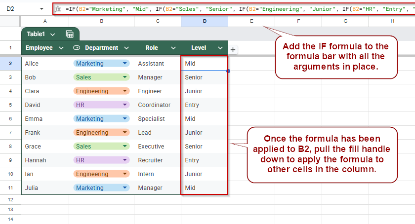
➤ In cell D2, enter the formula:
=IF(B2=”Marketing”, “Mid”, IF(B2=”Sales”, “Senior”, IF(B2=”Engineering”, “Junior”, IF(B2=”HR”, “Entry”, “”))))
➤ Drag the formula down from D2 to D11 to apply it to all rows.
Apply IF Logic to Update Cell Values
If you’re working with just a few drop-down options and want to display a related value in another column automatically, the IF formula is the simplest method. This approach is perfect when you have a small, fixed list of options, like department names, and you want to return a specific result (such as job level) based on what’s selected.
We’ll show you how to create a drop-down menu in the Department column, then use an IF formula to update the Level column automatically based on that selection.
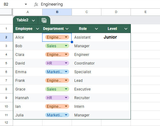
This is the dataset that we will be using to demonstrate the methods.
Steps:
➤ Select cells B2:B11.
➤ Go to Data >> Data validation
➤ Under Criteria, choose Drop-down.
➤ Google Sheets should automatically add the values from the selected range. If not, add the items, Marketing, Sales, Engineering, and HR.
➤ Click Done.
➤ In D2, enter this formula:
=IF(B2=”Marketing”, “Mid”, IF(B2=”Sales”, “Senior”, IF(B2=”Engineering”, “Junior”, IF(B2=”HR”, “Entry”, “”))))
➤ Drag this formula down from D2 to D11.

When you choose a department from the drop-down list, the corresponding level will automatically appear in the Level column.
Update Cell Values Using VLOOKUP in Google Sheets
If you’re working with many dropdown options or want a cleaner, more scalable solution, VLOOKUP is a great choice. This method uses a reference table to map each selection from the dropdown to a specific output value. When a user selects a department, the level column will automatically update by looking up the corresponding value from the table.
Using a lookup table, we’ll continue using the same employee dataset and update the Level column based on the selected Department.
Steps:
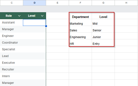
➤ In cells F1:G5, enter the following reference table:
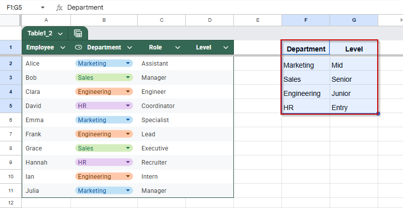
➤ Click cell D2 and enter this formula:
=IFERROR(VLOOKUP(B2, F$1:G$5, 2, FALSE), “”)
➤ Drag the formula down from D2 to D11 to apply it to the rest of the column.
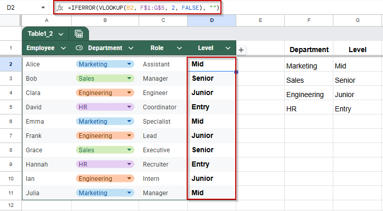
When a department is selected in Column B, the Level in Column D updates instantly using the mapping defined in your reference table.
Using SWITCH Formula to Update Cell Values Based on Drop-Down Selection
The SWITCH formula is a great alternative to using multiple IF statements. Instead of stacking many conditions, SWITCH lets you check one cell’s value and return different results based on exact matches. This method is useful when you have several known options (like department names) and you want a specific value (like job level) to appear automatically when one is selected from a drop-down list.
We’ll continue using the same dataset, where a department is selected in Column B. We want Column D (Level) to update automatically based on the department name.
Steps:
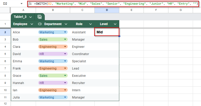
➤ Click on cell D2, where you want the result (Level) to appear.
➤ Enter the following formula:
=SWITCH(B2, “Marketing”, “Mid”, “Sales”, “Senior”, “Engineering”, “Junior”, “HR”, “Entry”, “”)
➤ Press Enter to confirm the formula.
➤ Click on the fill handle (small square at the bottom-right corner of the cell) and drag it down to fill D2 to D11.
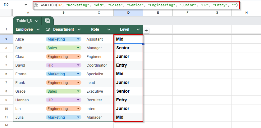
Now, as soon as you select a department from the drop-down in Column B, the correct level will automatically appear in Column D. The SWITCH formula keeps your sheet cleaner and is easier to edit than deeply nested IF formulas.
Automatically Update Cell Values Using Google Apps Script
If you want cell values to update instantly without formulas, Google Apps Script is the most flexible and powerful method. With just a few lines of code, you can create a script that automatically fills in related cell values when someone selects an option from a drop-down list.
This method is ideal when you want behind-the-scenes automation. For example, when someone chooses a department in Column B, the script will immediately enter the correct level in Column D. No formulas are required, and it updates in real time.
Steps:
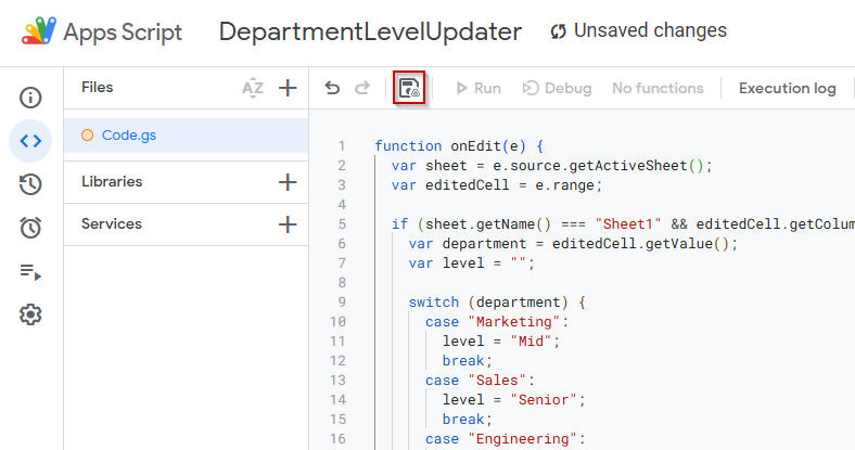
➤ Open your Google Sheet and make sure the sheet name is “Sheet1” (or change it in the script later if needed).
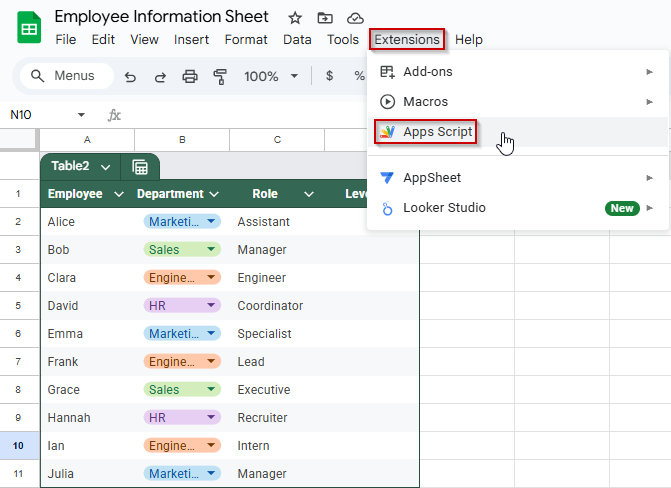
➤ Go to Extensions >> Apps Script to open the script editor.
➤ Delete any code that’s already there to start fresh.
➤ Copy and paste the following script into the editor:
function onEdit(e) {
  var sheet = e.source.getActiveSheet();
  var editedCell = e.range;
  if (sheet.getName() === "Sheet1" && editedCell.getColumn() === 2) {
    var department = editedCell.getValue();
    var level = "";
    switch (department)
      case "Marketing":
        level = "Mid";
        break;
      case "Sales":
        level = "Senior";
        break;
      case "Engineering":
        level = "Junior";
        break;
      case "HR":
        level = "Entry";
        break;
    }
    sheet.getRange(editedCell.getRow(), 4).setValue(level); // Column D
  }
}
➤ Click the floppy disk icon or go to File >> Save, and give your project a name like DepartmentLevelUpdater.
➤ Close the Apps Script tab and return to your spreadsheet.
➤ Test your script by selecting a department from the drop-down in Column B.
The corresponding level will instantly appear in Column D, automatically.
Change Cell Values Using INDEX-MATCH Formula
The INDEX and MATCH functions find and return specific values from a dataset based on a user’s selection. This method helps pull in related information, such as a job level or role, based on a dropdown selection like department. Unlike VLOOKUP, INDEX and MATCH are more flexible with column positions and can work with data in any orientation.
We’ll use a reference table to match each department to its corresponding level, then automatically return that value in a new column when a department is selected from the dropdown.
Steps:
➤ Create a separate reference table in the range F1:G5.
➤ Click on cell D2
➤ Enter this formula:
=IFERROR(INDEX(G$2:G$5, MATCH(B2, F$2:F$5, 0)), “”)
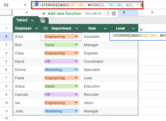
➤ Press Enter.
➤ Drag the formula down from D2 to D11
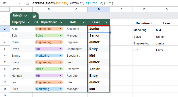
This will find the first matching department from column B and return the Level from column D.
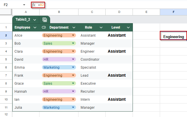
Change Cell Values Based on Dropdown Selection Using TRANSPOSE and FILTER Functions
The TRANSPOSE and FILTER functions let you extract all matching values based on a dropdown selection and display them across a row (horizontally) or column (vertically). This is helpful when showing all roles or levels tied to a specific department rather than just one result. For example, if a department like “Engineering” has multiple employees with different roles, this method can return all of them in one line.
Steps:
➤ Select cell F2 and link it directly to a dropdown cell such as B2 with =B2.
➤ Click cell G2 and enter the following formula:
=TRANSPOSE(FILTER(C2:C11, B2:B11=F2))
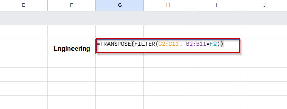
➤ Press Enter to apply the formula.
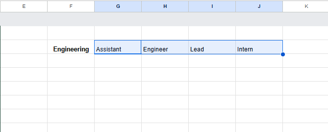
➤ Try changing the value in B2 from Engineering to HR by selecting from the dropdown.
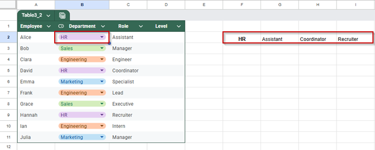
Now, whenever you select a department from the dropdown, the corresponding roles will appear starting from G2 and be displayed horizontally. If you prefer a vertical layout, simply remove the TRANSPOSE function and use only FILTER.
Frequently Asked Questions
How can I automatically populate a cell based on a dropdown selection in another cell?
Use the VLOOKUP function with a reference table to return values based on a drop-down input. When a selection is made from the drop-down, it updates the target cell instantly.
What is the difference between using IF, SWITCH, and VLOOKUP for updating cell values based on dropdowns?
IF works best for a few options. SWITCH is cleaner for multiple exact matches. VLOOKUP is ideal for larger lists and keeps formulas short by referencing a separate table.
Can I update cells in another sheet based on a dropdown selection?
Yes. Use VLOOKUP or INDEX/MATCH functions with cross-sheet references to update values. This allows dynamic updates between sheets based on dropdown selections in the main sheet.
How can I display multiple results based on a single dropdown selection?
Use the FILTER function to return all matching values, and the TRANSPOSE function to adjust the layout. This is useful for showing multiple results related to one dropdown category.
Wrapping Up
Automatically updating cell values based on dropdown selections can make your spreadsheets more interactive, efficient, and user-friendly. Whether assigning levels to departments, mapping roles, or pulling data from a reference table, these methods reduce manual work and improve data accuracy.
With just a few steps, you can build smarter spreadsheets that respond to user input instantly, making them ideal for dashboards, reports, or data entry systems. Try each method with your dataset to see what works best for your needs.