How to Extract a URL from a Hyperlink in Google Sheets

If you’ve added or imported data into Google Sheets, sometimes you’ll notice that a cell shows clickable text (like “Click here”), but it actually links to a different website in the background. If you want to pull out only the URL from that hyperlink, not the display text, there are a few simple ways.

This article explains how to extract URLs from link-formatted cells using built-in functions, formulas, and Google Apps Script.

Key Takeaways

Steps to Extract URLs from Rich Text Links Using Apps Script in Google Sheet

➤ Use Google Apps Script when your cell contains rich text with hidden links (e.g. display text like "Visit site" with a clickable URL underneath).
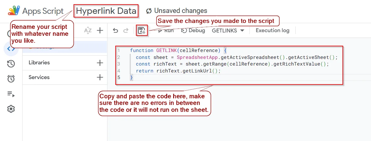
➤ Go to Extensions >> Apps Script in your Google Sheet to open the script editor.
➤ Delete any default code and paste this function:

VBA Code

Copy

function GETLINK(cellReference) {
  const sheet = SpreadsheetApp.getActiveSpreadsheet().getActiveSheet();
  const richText = sheet.getRange(cellReference).getRichTextValue();
  return richText.getLinkUrl();
}

➤ Save the script by clicking the disk icon or going to File > Save. You can give the project any name.
➤ Back in your sheet, use the custom formula like this: =GETLINK("D2") This will extract the hidden URL from cell D2.

The REGEXEXTRACT function in Google Sheets lets you pull specific text from a string using a pattern. When hyperlinks are added using the HYPERLINK function, the URL is stored inside that formula and is not visible in the cell unless you extract it.

By combining REGEXEXTRACT with FORMULATEXT, you can search inside the formula and pull out just the link. This method works when the hyperlink was written directly using the formula's full URL, not cell references.

In this case, the URL is stored right inside the formula. Google Sheets won't show it in the cell, but we can extract it using REGEXEXTRACT.

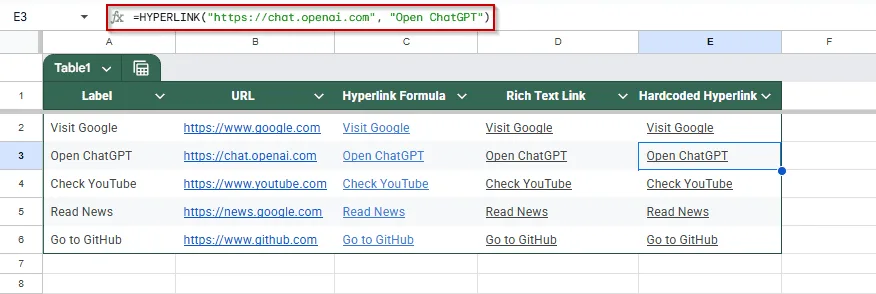
We’ll use this method on the Hyperlink Data sheet, specifically column E, where each cell contains a formula like: =HYPERLINK("https://www.google.com", "Visit Google")
Steps:

➤ Go to cell F1
➤ Enter this formula:

➤ Press Enter. This extracts the full URL from the hyperlink in A1.

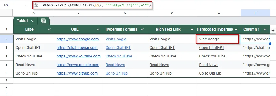
➤ Drag the formula down to extract links from A2 through A5.

When hyperlinks are created in Google Sheets using the HYPERLINK function, the URL itself is often hidden, either written directly as a string or pulled in from another cell reference. You won’t see the actual link unless you hover or click on it.

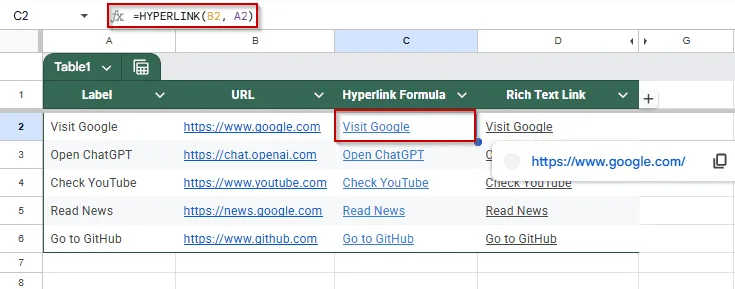
If your formula uses a cell reference, like: =HYPERLINK(B2, A2), you can’t extract the raw URL using REGEXEXTRACT alone because FORMULATEXT will return the formula as "=HYPERLINK(B2, A2)," not the actual URL.

➤ In your sheet, click the cell and look at the formula bar. If it starts with =HYPERLINK(...), you're good to go for this method.

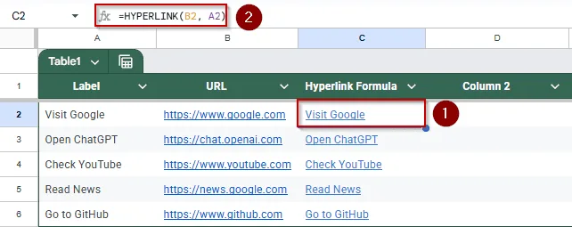
➤ Now, click on the cell next to it (e.g., D2 if the hyperlink is in C2).
➤ Enter this formula:

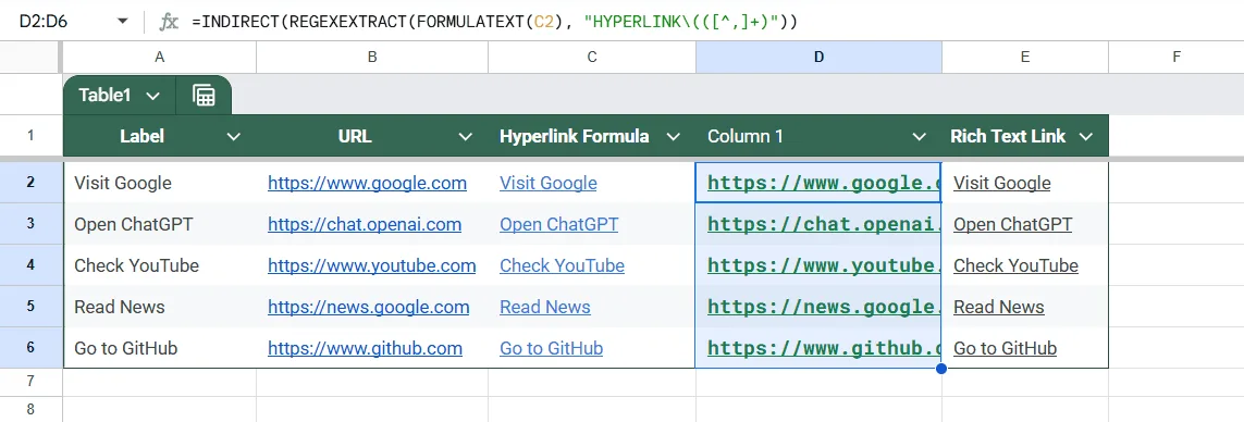
➤ Press Enter. You’ll see the URL from the hyperlink formula appear in the new cell.

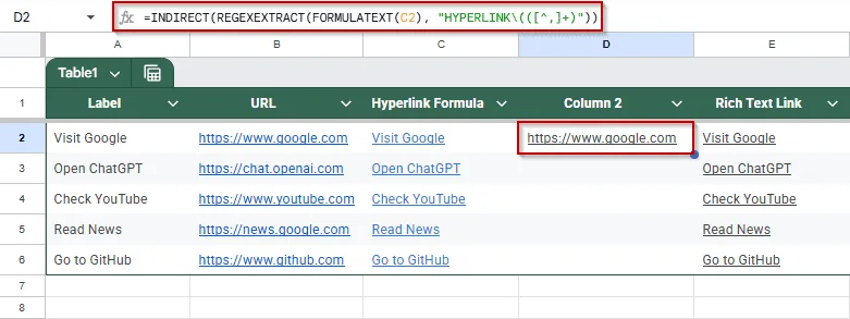
➤ You can now drag the formula down to apply it to other rows in the column.

If your cell has rich text, meaning the visible text says something like "Visit site", but the actual link is hidden behind it, Google Sheets doesn't have a built-in function to extract it. But you can create a simple Apps Script to do it.

Google Apps Script is a built-in coding tool in Google Sheets that lets you automate tasks, build custom functions, and access hidden data. It uses JavaScript and runs directly in your spreadsheet.

➤ In your sheet, click Extensions >> Apps Script from the top menu.

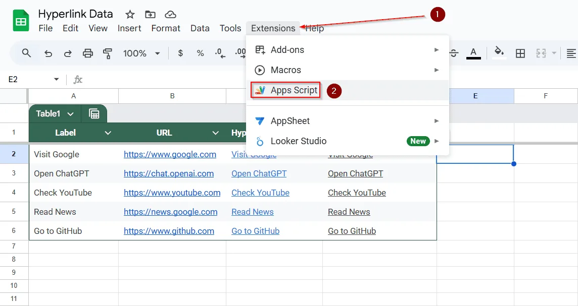
➤ A new tab will open. Delete any default code you see inside.
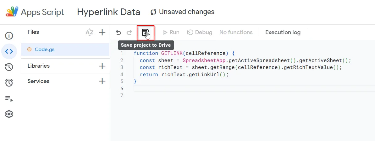
➤ Copy and paste this code:

function GETLINK(cellReference) {
  const sheet = SpreadsheetApp.getActiveSpreadsheet().getActiveSheet();
  const richText = sheet.getRange(cellReference).getRichTextValue();
  return richText.getLinkUrl();
}

➤ Click the disk icon or go to File >> Save. You can name the project anything you like.

➤ Now go back to your Google Sheet.
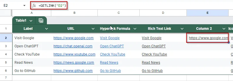
➤ In an empty cell, type:

➤ Press Enter. The actual URL behind the link in D2 will appear in the new cell.

If you have a long list of cells with manually added hyperlinks (rich text) and want to extract the URL from each of them all at once, the regular GETLINK function only works one cell at a time.

To speed up the process, you can use another custom Google Apps Script that extracts all URLs from a column in one go.

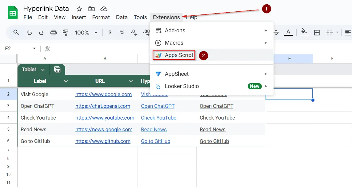
➤ In your sheet, click Extensions >> Apps Script.

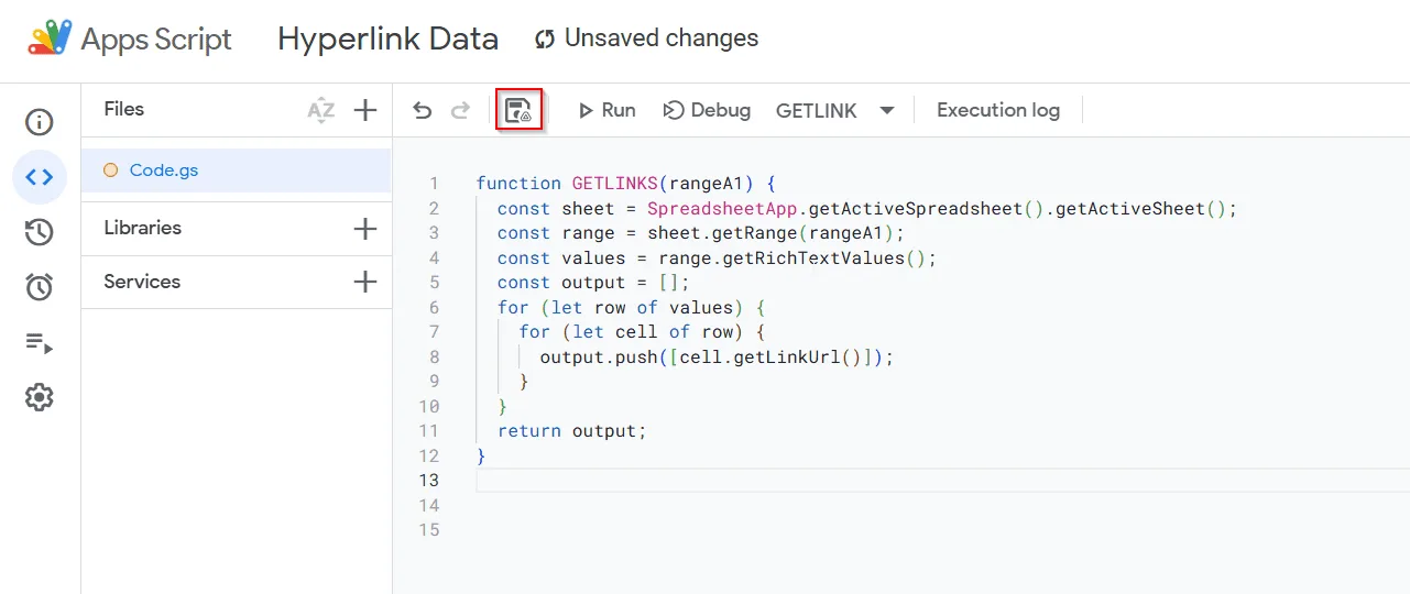
➤ Delete any default code and paste the following:

function GETLINKS(rangeA1) {
  const sheet = SpreadsheetApp.getActiveSpreadsheet().getActiveSheet();
  const range = sheet.getRange(rangeA1);
  const values = range.getRichTextValues();
  const output = [];
  for (let row of values) {
    for (let cell of row) {
      output.push([cell.getLinkUrl()]);
    }
  }
  return output;
}

➤ Click the disk icon or go to File >> Save, and name the project anything you like.

➤ Go back to your sheet and select an empty column.
➤ Type this formula:

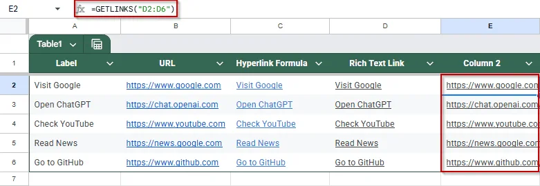
Each row will return the link behind the rich text in the corresponding cell.

Practice Resources

Get our practice workbook or necessary files that we have worked with to prepare this article.

Extract URL from a Hyperlink in Google Sheets [Make a Copy]

Frequently Asked Questions

You can extract URLs from rich text hyperlinks using Google Apps Script. You can create a custom function since Google Sheets doesn't provide a built-in function for this. Here's how:

➤ Go to Extensions >> Apps Script in your Google Sheet.
➤ Delete any existing code and paste the following:

function GETLINK(cellReference) {
  const sheet = SpreadsheetApp.getActiveSpreadsheet().getActiveSheet();
  const richText = sheet.getRange(cellReference).getRichTextValue();
  return richText.getLinkUrl();
}

➤ Click the disk icon or go to File >> Save to save the script.
➤ Back in your sheet, use the custom function like this: =GETLINK("A2")

This will extract the URL from the hyperlink in cell A2.

If your hyperlinks are created using the HYPERLINK function, you can extract the URL using a combination of FORMULATEXT and REGEXEXTRACT. Here's how:

➤ If your hyperlink formula is in cell A1, enter the following formula in another cell:

➤ Press Enter. This will extract the URL from the hyperlink formula in A1.

When you create a hyperlink using the HYPERLINK function with cell references, like =HYPERLINK(B2, A2), the actual URL is in cell B2. Using FORMULATEXT on such a cell returns the formula as text, not the evaluated URL.

Built-in functions like REGEXEXTRACT and FORMULATEXT can extract URLs from hyperlinks created using the HYPERLINK function with direct URLs. However, they don't work for hyperlinks added manually (rich text) or those made using cell references.

Yes, there are add-ons like "Links Extractor" available in the Google Workspace Marketplace. This add-on can extract texts and links from a specified range in your Google Sheet. To use it:

➤ Go to the Links Extractor add-on page.
➤ Click "Install" and follow the prompts to add it to your Google Sheets.
➤ Once installed, you can use it to extract hyperlinks from selected ranges.

Wrapping Up

If your Google Sheets contains hyperlinks and you need to extract the actual URLs, there’s more than one way to get it done. Whether the links are added by formula or inserted manually, you can use a combination of built-in functions or a short Apps Script to reveal what’s hidden behind the clickable text.

The REGEXEXTRACT function is excellent for quick, one-off extractions. The Apps Script method gives you the most flexibility for richer formatting or automation, especially when dealing with manually added links.