
How to Filter with Multiple Conditions in Google Sheets
Sometimes you may need to filter rows to help you control sales records, student grades, employee databases, or project files. However, there is one limitation of the default available sets of filters: it can be difficult to apply filters that meet two different criteria at the same time. That's where the FILTER function comes in. It is dynamic because it offers results on demand that change as your data does.
➤ AND Conditions: Use the asterisk (*) symbol to combine several conditions; so all conditions should be fulfilled for the rows under consideration.
Example:
=FILTER(A2:E13, (B2:B13="New York") * (C2:C13="Condo"))
➤ OR Conditions: The plus (+) symbol is what you need if you want to filter your rows when any one condition is true.
In this article, we will talk about some easy ways to Filter Multiple Conditions in Google Sheets: FILTER function with AND logic, FILTER function with OR logic, filtering with text and numeric conditions combined, QUERY function with multiple conditions, filtering with partial text (case sensitive and insensitive), etc.
How Does FILTER Function Work in Google Sheets?
The FILTER function in Google Sheets removes subsets of data from a chosen data range under a given criteria based on condition. Unlike the built-in filter tool, which visually hides rows, the FILTER function creates a new dynamic range where only the matching rows are displayed.
Here’s the syntax:
=FILTER(range, condition1, [condition2, ...])Let’s look at an example here. We're going to filter the data based on a particular text "Condo". As a result, rows containing Condo in Column C will appear in the result.
=FILTER(A2:E13, C2:C13="Condo")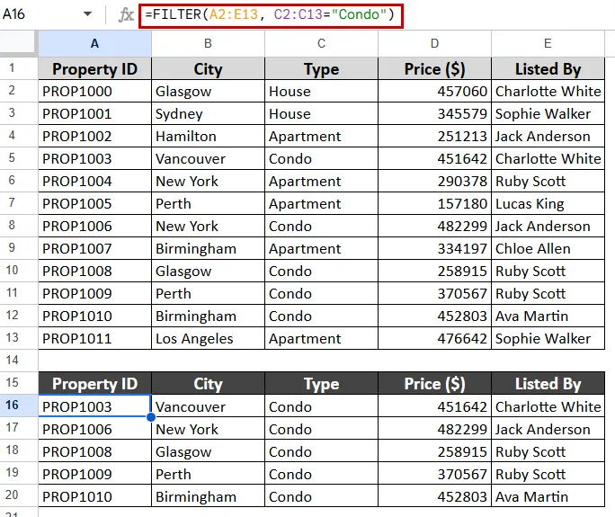
Using the FILTER Function with AND Logic
The FILTER function makes it possible to combine conditions with the asterisk (*_ operator (which is equivalent to AND in logic). The general formula of AND logic:
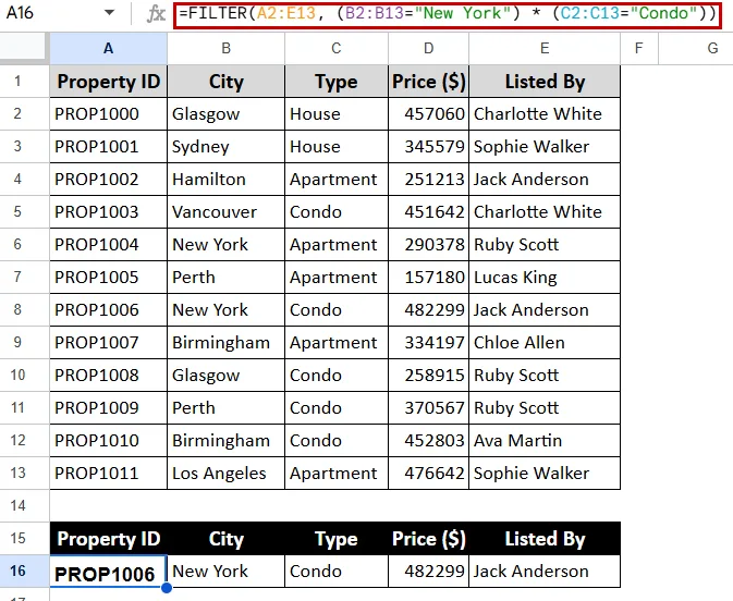
=FILTER(range, (condition1) * (condition2))Suppose we want to filter only the properties in New York and Condos.
➤ Select a blank cell where the filtered result will begin. Here we select F2.
➤ Enter the formula using asterisk (*) between each condition.
=FILTER(A2:E13, (B2:B13="New York") * (C2:C13="Condo"))➤ Press Enter. And here’s the result
Using the FILTER Function with OR Logic
If the OR logic is applied, the FILTER function will return all rows where at least one of the conditions is met.
Here’s the formula:
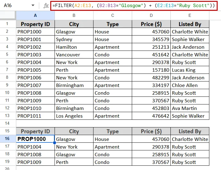
=FILTER(range, (condition1) + (condition2))Let's say we want to filter properties that are either in Glasgow or owned by Ruby Scott. We can use the (+) plus sign (OR) as FILTER for performing logical OR conditions.
➤ Select a blank cell (for example, F2).
➤ Enter the formula using + to separate the conditions:
=FILTER(A2:E13, (B2:B13="Glasgow") + (E2:E13="Ruby Scott"))➤ Press Enter to get the filtered result.
Filtering with Text and Numeric Conditions Combined
You might need to filter using both text and numeric criteria—for example, showing entries from a certain region and a sales value above a specific threshold.
Here’s the formula:
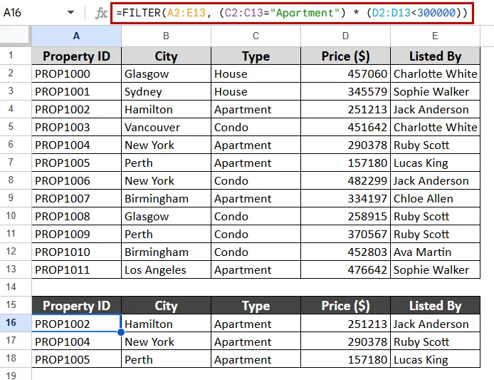
=FILTER(range, (column="value") * (column<number))Suppose you want to filter all Condos that are priced above 400,000.
➤ Select a blank cell. Here we select F2.
➤ Enter the formula:
=FILTER(A2:E13, (C2:C13="Apartment") * (D2:D13<300000))➤ Press Enter and find out the results.
Filtering Based on Multiple Columns with Mixed Logic
Depending on the column numbers, you can mix conditions inside the FILTER function using * for AND and + for OR with mixed logic.
Here’s the formula:
=FILTER(range, ((condition1) + (condition2)) * (condition3))Let’s assume you want to filter properties owned by Ruby Scott in Perth OR New York.
➤ Select a blank cell. Here we select F2.
➤ Enter the formula:
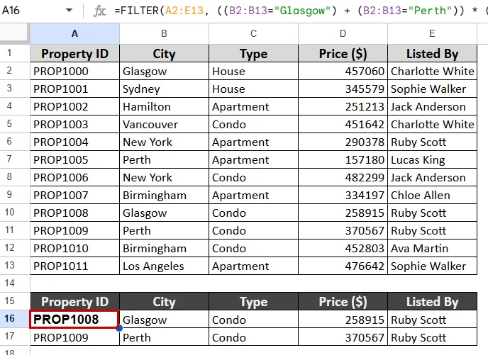
=FILTER(A2:E13, ((B2:B13="Glasgow") + (B2:B13="Perth")) * (E2:E13="Ruby Scott"))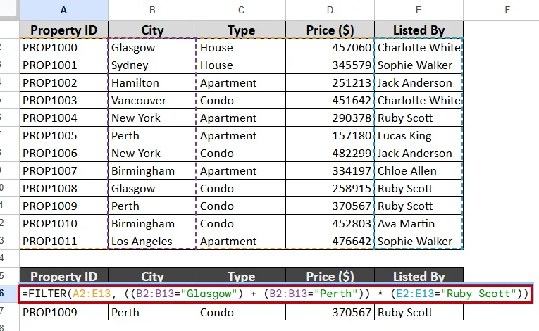
➤ Press Enter. Here are the results you will see.
Using the QUERY Function with Multiple Conditions
The QUERY function provides SQL-like syntax to search Google Sheets and more freedom for sophisticated filtering.
Here’s the formula:
=QUERY(range, "SELECT * WHERE condition1 AND/OR condition2", -1)Example 1: AND Logic
Apartments in Birmingham:
➤ Select a blank cell (e.g. F2).
➤ Enter the formula:
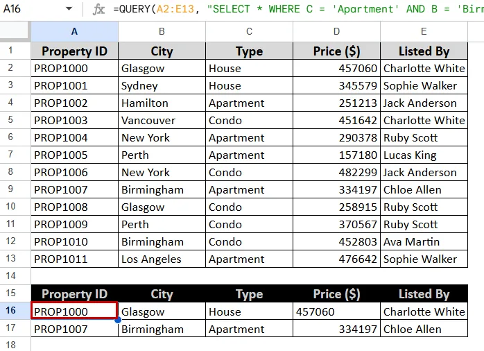
=QUERY(A2:E13, "SELECT * WHERE C = 'Apartment' AND B = 'Birmingham'", 1)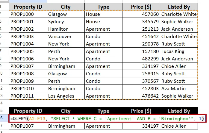
➤ Press Enter to get the filtered result.
Example 2: OR Logic
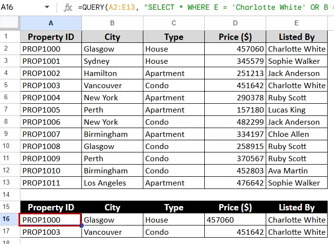
Properties listed by Charlotte White or in Vancouver:
➤ Select a blank cell (e.g. F2).
➤ Enter the formula:
=QUERY(A2:E13, "SELECT * WHERE E = 'Charlotte White' OR B = 'Vancouver'", 1)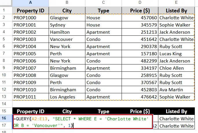
➤ Press Enter and find out the results
Filtering with Partial Text (Case-Insensitive)
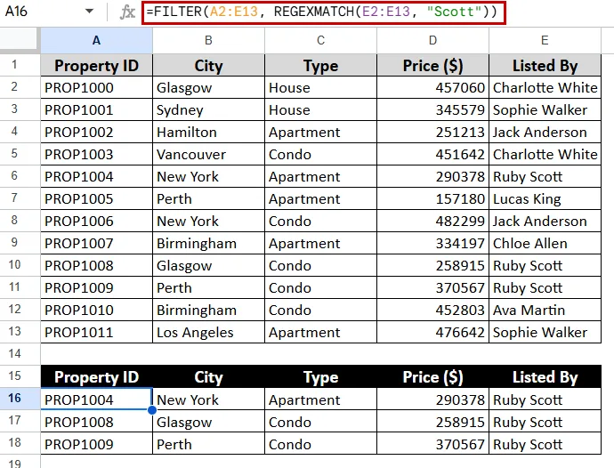
With Google Sheets, the REGEXMATCH() function lets you filter rows depending on whether a particular text—regardless of letter case—is found within a cell.
Here’s the formula:
=FILTER(range, REGEXMATCH(range, "partial_text"))Suppose you want to filter properties whose owner name includes "Scott."
➤ Select a blank cell (example F2).
➤ Enter the formula:
=FILTER(A2:E13, REGEXMATCH(E2:E13, "Scott"))➤ Press Enter and find out the results
Filtering with Partial Text (Case-Sensitive)
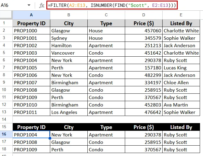
Use the FIND function within the FILTER formula if you want the filter to be case-sensitive, that is to match the exact casing of the search term.
Here is the formula:
=FILTER(range, ISNUMBER(FIND("partial_text", range)))And now you want to find the owner named “Scott” and not “scott” or “SCOTT”.
➤ Select a blank cell (example F2).
➤ Enter the formula:
=FILTER(A2:E13, ISNUMBER(FIND("Scott", E2:E13)))➤ Press Enter and find out the results
Filter Multiple Conditions without Using Formulas
Without creating any formulas, Google Sheets also offers a built-in way to filter data depending on several criteria. You can do this with the Create a filter tool.
➤ Select your data range (e.g., A1:E13).
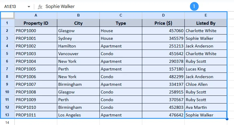
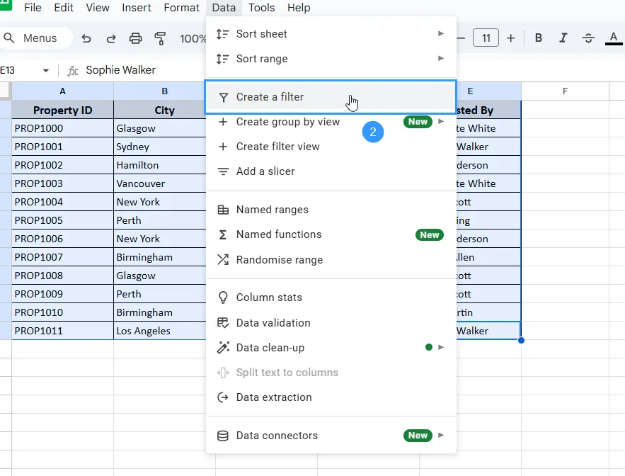
➤ Go to the Data menu and click on Create a filter.
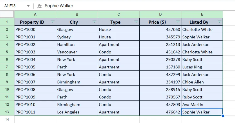
➤ Little green filter icons will appear in each column header.
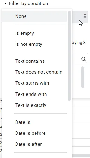
➤ Click the filter icon on the desired columns to apply Filters by condition.
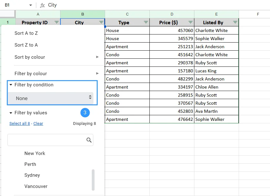
➤ There are various conditions available for you to choose from. Choose any to find out.
Practice Resources
Get our practice workbook or necessary files that we have worked with to prepare this article.
Filter with Multiple Conditions in Google Sheets [Make a Copy]
Frequently Asked Questions
What happens if the filter returns no matching results?
The FILTER function will give you a #N/A error if none of the properties in your dataset meet the filtering requirements. To handle this easily, wrap it in IFERROR like this:
=IFERROR(FILTER(range, (condition1) * (condition2) * ...), "No matching results")This will display "No matching results" instead of an error.
Can I filter data across multiple sheets?
Yes, you can filter data across multiple sheets. Use the formula:
=FILTER(range, condition1, condition2, ...)Can I filter rows that match one of many values?
Yes. You can use the =ISNUMBER(MATCH()) combination to filter rows that match one of many values.
How can I sort filtered results?
Though you can wrap the FILTER function inside the SORT function, it does not sort results by itself. Here’s the formula:
SORT(FILTER(range, condition1, [condition2, ...]), sort_column, is_ascending)
Concluding Words
Working with complicated data is quite simple when you can use FILTER function over several sheets. This approach helps you to rapidly and effectively extract particular data whether you are handling real estate listings or any other dataset. It's a basic but efficient approach to maintain your analysis clear and concentrated.
Related Google Sheets Basics Articles
Master the fundamentals with these step-by-step spreadsheet tutorials















Liked this lesson? Get one practical spreadsheet tip every week.
Comments
No comments yet — be the first to ask a question.