Polynomial interpolation is a useful approach when working with non linear data and trying to estimate values between known data points. Excel offers built in features that will help you interpolate with a few manual steps. In this tutorial, we’ll teach you the basics of polynomial interpolation, how to perform polynomial interpolation in Excel. Using a simple dataset, we’ll walk through the steps so you can confidently apply this technique to your data.
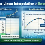
➤ Polynomial interpolation fits a polynomial function to estimate values from known data. In this article, we’ll learn about polynomial interpolation and show the steps to perform polynomial interpolation in Excel using the Trendline feature and Matrices.
➤ Trendline: Insert Chart >> Chart Elements >> Trendline >> More Options >> Display equation on chart >> Plug in x value.
➤ Matrices: Choose order of the polynomial >> Set up the matrix of powers >> Create column vector >> Solve matrix equation for coefficients >> Construct polynomial equation >> Plug in x value.
➤ Solving for coefficients: =MMULT(MINVERSE(cell_reference), cell_reference)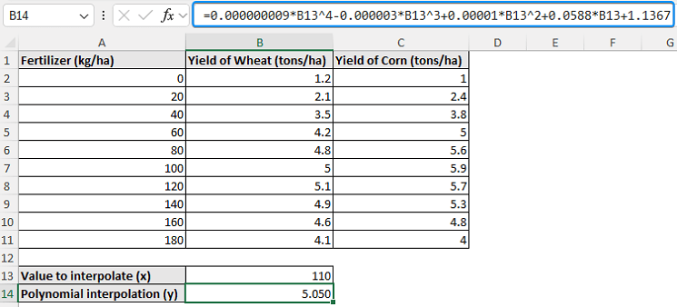
What Is Polynomial Interpolation in Statistics?
Polynomial interpolation fits a single polynomial curve through all of the data points. While linear interpolation connects points with straight lines. This method is well suited for datasets that display a nonlinear trend. The general form of a polynomial function with n data points is:
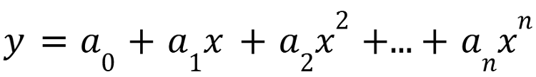
where a0,a1,a2…an are coefficients to be determined.
Polynomial Interpolation in Excel with Trendline
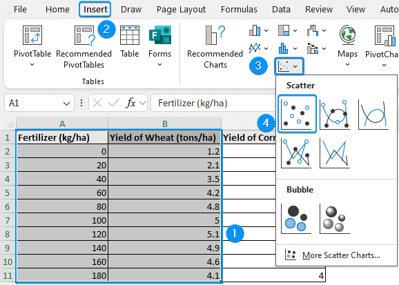
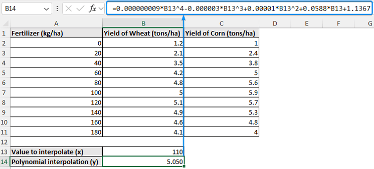
Consider the crop yield vs. fertilizer dataset containing the fertilizer (kg/ha), yield of wheat (tons/ha), and yield of corn (tons/ha) in columns A through C.
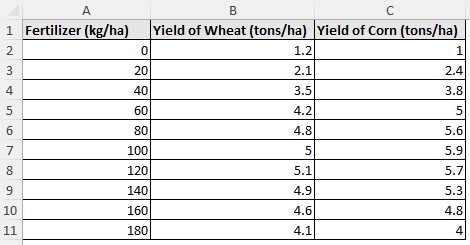
In this dataset, the crop yield (dependent variable) is influenced by the use of fertilizer (independent variable).
Let’s say you are calculating the wheat and corn yields at 110 kg/ha of fertilizer. Due to the non linear trend of this dataset, a polynomial interpolation will offer a more accurate estimation than linear interpolation between 100 and 120 kg/ha.
The Trendline approach fits a curve through the data points using Excel’s polynomial Trendline feature to estimate wheat production at an intermediate fertilizer level (110 kg/ha). This method is suitable for a fast visual representation without much calculation. Furthermore, the use of the complete dataset can reveal a broader trend.
Steps:
➤ Select the data range (A1:B11) >> Insert >> Scatter or Bubble Chart >> Scatter.
➤ Click Chart Elements >> Uncheck Gridlines >> Enable Trendline >> More Options.
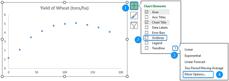
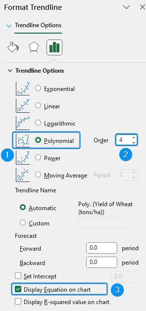
➤ Select Polynomial Trendline >> Adjust the Order until best fit through the data points. For example, we’ve chosen order 4 >> Check the Display equation on chart option.
➤ Select the polynomial equation >> Press Ctrl + C to copy.
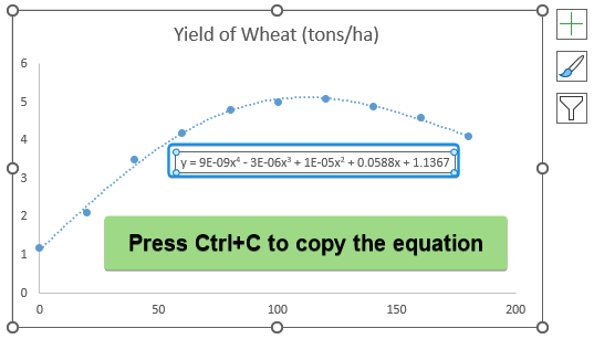
➤ Paste the equation in cell B14 >> Plug in the x value (110 kg/ha fertilizer) to calculate the y value (wheat yield).
The discussion and key findings of the results are covered after the second approach.
Polynomial Interpolation in Excel with Matrices
The matrices method uses Excel’s MMULT and MINVERSE to solve algebraic equations and obtain the coefficients of the polynomial function. A fourth order polynomial offers flexibility and precision for the polynomial interpolation. Although this method requires prior knowledge of matrices and is somewhat challenging to set up, it is convenient and well suited for custom applications and accurate modeling.
Steps:
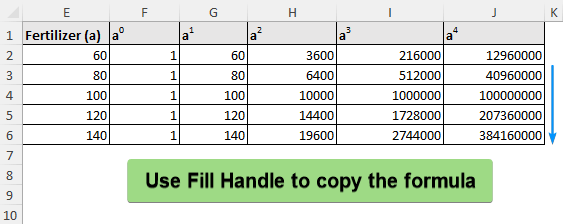
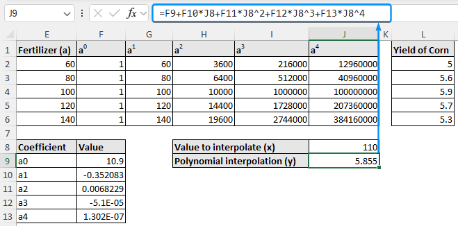
➤ To fit a 4th order polynomial, we need 5 data points. Select five data points from the fertilizer column surrounding the targeted interpolation value (110). For example, we created the column “Fertilizer (a)” and chose the data points 60, 80, 100, 120, and 140.
➤ Create columns for a0 to a4 >> Calculate the value of “a” raised to the power of 0 to 4.
=E2^0=E2^1=E2^2=E2^3=E2^4

➤ Use Fill Handle to auto fill the table.
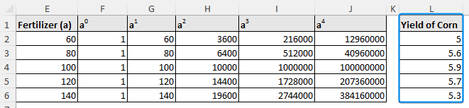
➤ Make a column vector with the corn yield values corresponding to the chosen data points.
➤ Solve for the coefficients using matrix multiplication >> For earlier versions of Excel, press Ctrl + Shift + Enter or hit Enter for newer versions of Excel.
=MMULT(MINVERSE(F2:J6),L2:L6)
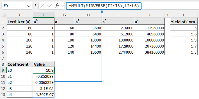
➤ Using the coefficients, construct the polynomial equation >> Plug in the x value (110 kg/ha fertilizer) to estimate the y value (corn yield).
=F9+F10*J8+F11*J8^2+F12*J8^3+F13*J8^4
➤ Using the equation of this curve, we performed polynomial interpolation to estimate intermediate values.
➤ For the second approach, we used matrices to solve a series of equations and obtain the coefficients of the polynomial functions. Using this function, we estimated an intermediate value.
➤ For 110 kg/ha of fertilizer, the estimated wheat yield is 5.05 tons/ha.
➤ For 110 kg/ha of fertilizer, the estimated corn yield is 5.86 tons/ha.
Trendline vs. Matrices: Pros and Cons
| Feature | Trendline | Matrices |
|---|---|---|
| Ease of use | Very easy to use | Setting up the matrices and use of Excel formulas |
| Order of the equation | 2 to 6 | Any order limited by Excel’s computational power |
| Repeatability | Not as easily repeatable for a different value of x | Once set up can be repeated for other values of x |
| Suitable for | Quick estimation and visualization of the trend | Accurate and detailed modeling |
| Limitation | Requires manual setup of the equation | Requires knowledge of matrices and algebra; Difficult to set up the matrices |
FAQ
How do I add a polynomial trendline in Excel?
Select the dataset >> Insert a Scatter plot >> Click on Chart Elements >> Go to Trendline >> More Options >> Polynomial.
How do you perform bilinear interpolation in Excel?
➤ Identify the x1,x1,y1, and y2 values from a table.
➤ Calculate the F11, F12, F21, and F22 values.
➤ Plug in these values in the bilinear interpolation formula.
Why use a polynomial trendline?
A polynomial trendline is suitable for data with a nonlinear trend.
How do you perform nonlinear interpolation in Excel?
Use the GROWTH function: <strong>=GROWTH(known_ys,[known_xs],[new_xs],[const])</strong>Or,
Insert Chart >> Chart Elements >> Trendline >> More Options >> Display equation >> Plug in x value.
What is the difference between interpolation and regression?
Interpolation joins each data point and is used to estimate an intermediate value based on known data points. Whereas, regression fits a curve of best fit to model the relationship between the variables and predict values beyond the known data range.
Wrapping Up
In this tutorial, we’ve taught you the basics of polynomial interpolation and how to perform polynomial interpolation in Excel using Trendline and matrices. Moreover, we’ve discussed the findings and compared the pros and cons of the two approaches. Feel free to download the practice file and share your thoughts and suggestions.