If your Excel sheet is filled with a long list of entries, finding and analyzing similar items can be overwhelming. Grouping similar items whether by text labels, categories, or numeric ranges makes your data cleaner and easier to summarize. Luckily, Excel offers several quick ways to group similar items.
In this article, you’ll learn simple to advanced methods to group similar items in Excel using built-in tools and formulas. Each method includes a step-by-step breakdown and sample data so you can follow along easily.
Steps to group similar items in Excel:
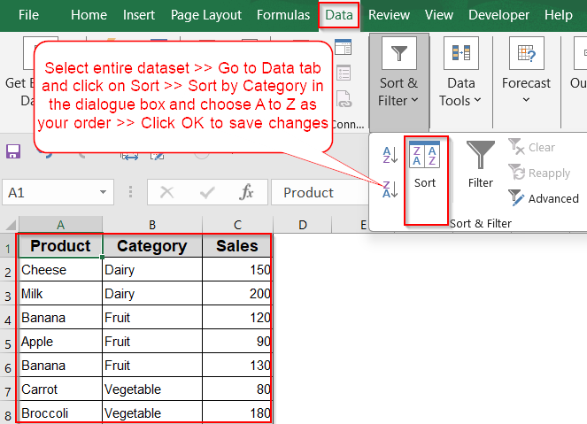
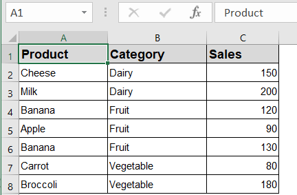
➤ Select your entire dataset (A1:C8 in this example).
➤ Go to the Data tab on the ribbon.
➤ Click on Sort under Sort & Filter drop-down.
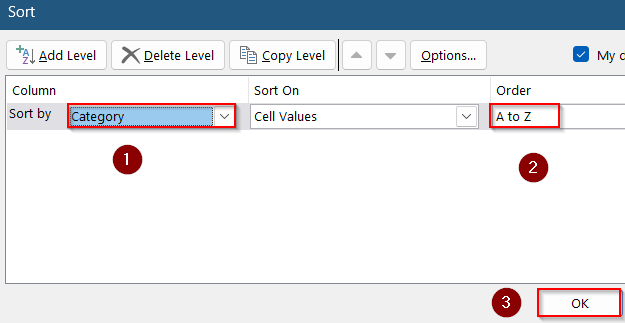
➤ In the dialog box, choose Category under Sort by and set A to Z as the Order.
➤ Click OK.
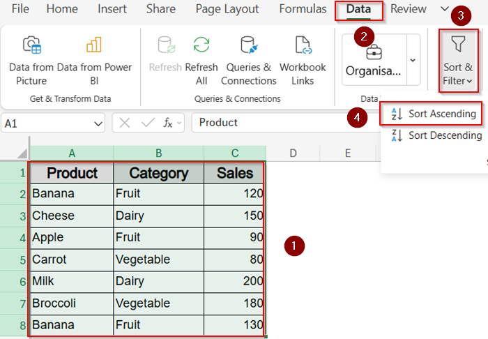
Sort Data to Visually Group Similar Items
Sorting your data is the simplest way to group similar items together. This doesn’t summarize data, but visually groups matching values side-by-side.
Steps:
➤ Select your entire dataset (A1:C8 in this example).
➤ Go to the Data tab on the ribbon.
➤ Click on Sort under Sort & Filter drop-down.
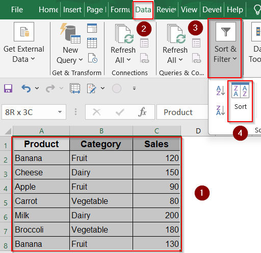
➤ In the dialog box, choose Category under Sort by and set A to Z as the Order.
➤ Click OK.
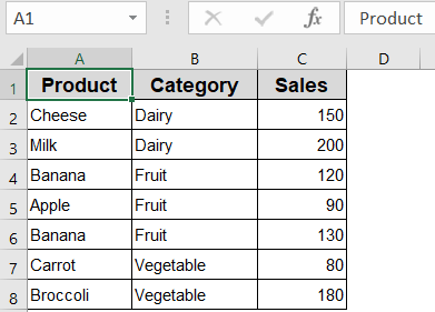
Now all similar categories (e.g., Dairy, Fruits, Vegetables) are grouped together alphabetically in your sheet.
Use Pivot Table to Group and Summarize Data
When you want to summarize data like total sales per category or product, Pivot Tables are the most powerful option. This method allows you to group items dynamically and aggregate numbers without altering your original dataset.
Steps:
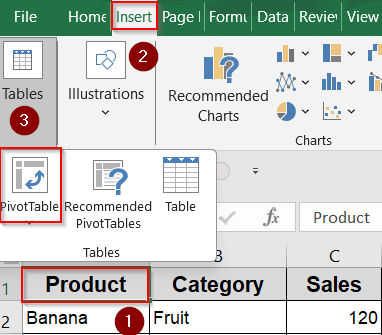
➤ Click anywhere in your dataset such as A1 cell.
➤ Go to the Insert tab >> Click PivotTable under the Tables group on the ribbon.
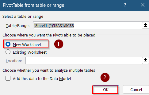
➤ Choose where to place the Pivot Table (e.g., New Worksheet) and click OK.
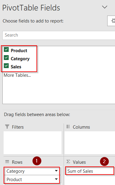
➤ In the Pivot Table Fields pane, drag Category to the Rows area and Sales to the Values area.
➤ Optionally, drag Product under Category to see grouped items.
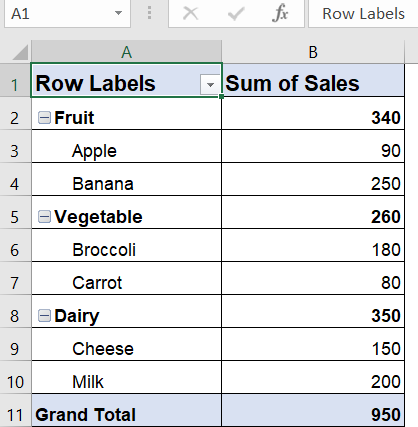
You’ll now see similar items grouped under their respective categories, along with total sales per group.
Automatically Group and Add Totals Using Subtotal Feature
The Subtotal feature lets you insert automatic grouping and totals every time a group changes which is great for grouped sales reports. It also provides collapse/expand controls for quick navigation through grouped blocks.
Steps:
➤ First, sort your data by Category (follow Method 1).
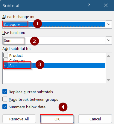
➤ Then go to the Data tab >> Click Subtotal under the Outline group.
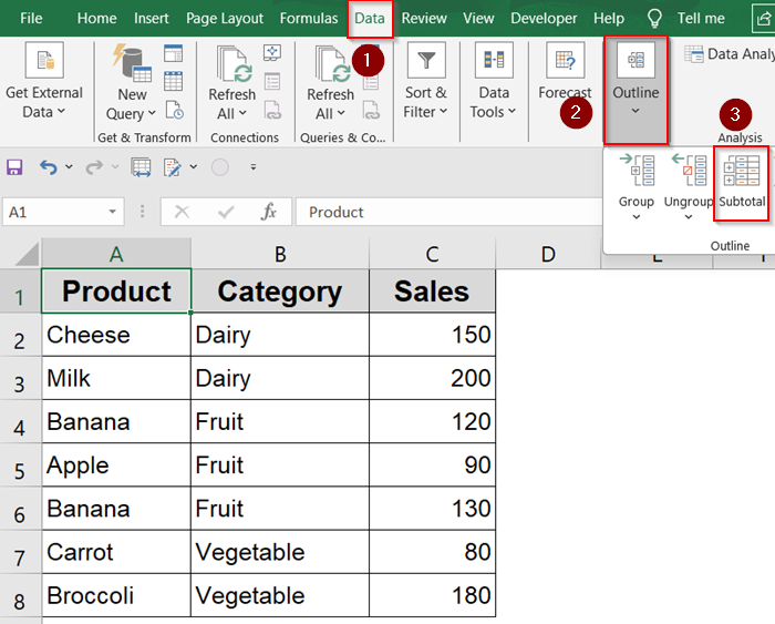
➤ In the dialog box, choose Category for At each change in, Sum for Use function , Sales for Add subtotal to field.
➤ Click OK.
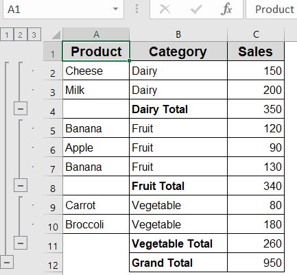
Excel will group the items by Category and insert subtotal rows for each group, with collapse/expand options on the left.
Count Unique Products by Category Using GROUPBY
This method uses Excel’s new GROUPBY function to count how many times each product appears within each category. It’s particularly helpful when you want a quick summary of repeated entries without using a pivot table.
In this example, we’ll calculate how many times each product shows up in its respective category using the GROUPBY function with a counting logic built inside.
Steps:
➤ Select a blank cell where you want to display the grouped result. For example, you can click on cell E2 to start the output in a new area.
➤ Type the following formula into the selected cell:
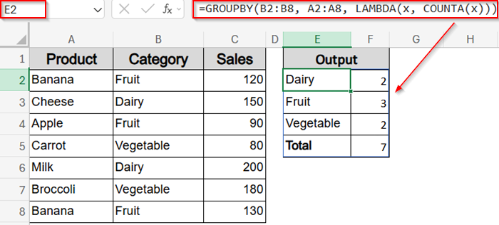
=GROUPBY(B2:B8, A2:A8, LAMBDA(x, COUNTA(x)))
Here, we’re grouping the data by Category column (B2:B8) and counting how many times items from Product column (A2:A8) appear using the LAMBDA and COUNTA functions inside the GROUPBY formula.
➤ Press Enter. Excel will instantly return a list where each category appears once, along with a count of how many times products are listed under it.
Return List of Items Instead of Count
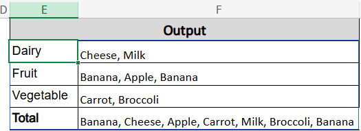
Instead of counting how many items appear under each category, this method shows the actual list of products for each category in a single, comma-separated line. It helps when you want to visually understand which items fall under each group.
Steps:
➤ Click on a blank cell where you want to begin the results. Let’s say you select cell E2.
➤ Paste the formula below into the selected cell:
=GROUPBY(B2:B8, A2:A8, LAMBDA(x, TEXTJOIN(“, “, TRUE, x)))
Here, the range B2:B8 contains categories we want to group by. A2:A8 holds the product names we want to return. The LAMBDA function uses TEXTJOIN to combine all products in each category into one comma-separated string.
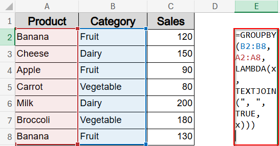
➤ Hit Enter. Excel will now output each category once, followed by a list of all products associated with that category.
Visually Group Rows by Product Name
If you want to visually group similar items, like all “Banana” entries, use Excel’s Group feature. This is useful for collapsing or expanding data for a specific product.
Steps:
➤ Select your entire dataset including headers (A1:C8).
➤ Go to the Data tab on the ribbon.
➤ Click on Sort Ascending under the “Sort & Filter” group (ensure the cursor is in the Product column) to group similar items.
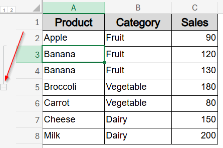
➤ Select row 3 and 4 with Banana entries, go to the Data tab >> In the Outline group, choose Group Rows under the Group button. You can also Group Columns if needed.
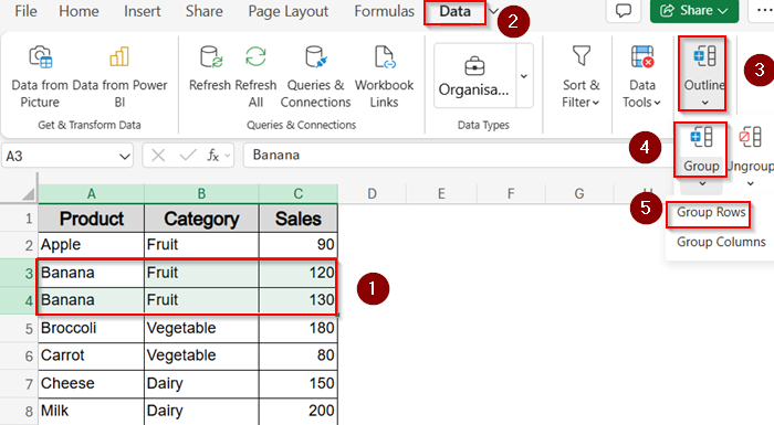
This allows you to collapse or expand grouped rows using the plus/minus button on the left. You can repeat the process for other products like Dairy items or Vegetables.
Extract Core Group Names Using a Formula
In some cases, your data may include minor variations (e.g., Apple fresh, Apple red). If so, you can extract the core product name using a formula to group them consistently.
Steps:
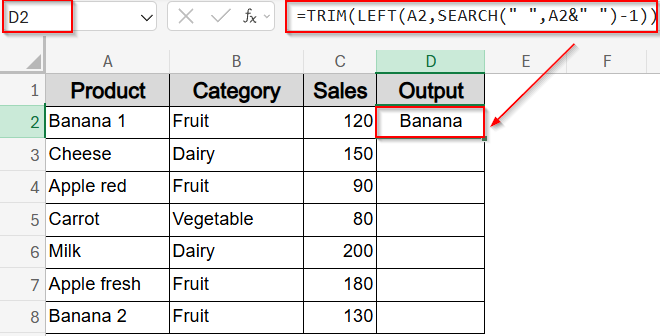
➤ Assume your data starts from A2 cell. Use this formula in D2 cell to remove extra identifiers and extract the base product:
=TRIM(LEFT(A2,SEARCH(” “,A2&” “)-1))
➤ Drag the formula down using the Autofill handle to apply it to all items.
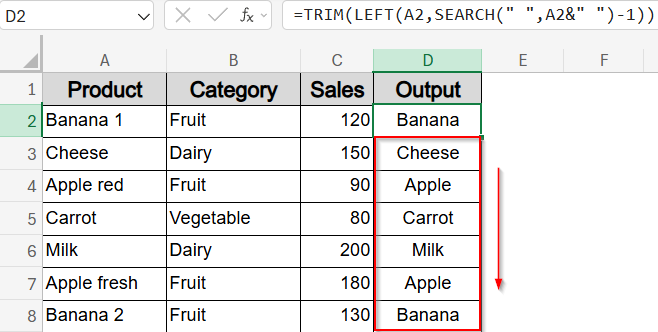
This will extract just the first word (e.g., “Banana”, “Apple”), making it easier to group later using sorting or pivot tables.
List Unique Product Names Using UNIQUE Function
If you want a clean list of unique products (no duplicates), Excel’s UNIQUE function is your best option.
Steps:
➤ Assume your data range is A2:A8. Select a blank cell (e.g., D2) and type formula:
=UNIQUE(A2:A8)
➤ Press Enter and Excel will immediately return distinct product names.
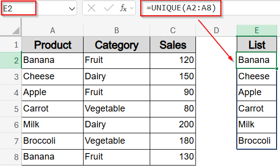
This is helpful when you need to create summaries or dropdown lists without duplicates.
Frequently Asked Questions
Can I group items by partial matches or similar text?
Not directly. If you want to group items by partial matches or similar text such as “Apple” and “Apples“, you’ll need to clean your data first using functions like TEXT, LOWER, TRIM, or use helper columns to standardize names before grouping.
Can I group data based on numeric ranges?
Yes. To group data based on numeric ranges like 0–100 or 101–200, add a helper column with formulas like: =IF(C2<=100, “0-100”, IF(C2<=200, “101-200”, “201+”)). Then group based on that column using a Pivot Table.
How do I ungroup items after using Subtotal?
If you wish to ungroup items after using the Subtotal feature, go to the Data tab on the ribbon and click on Subtotal. Then click Remove All.
Wrapping up
In this tutorial, we explored multiple ways to group similar items in Excel which start from basic sorting to advanced functions like GROUPBY and UNIQUE. Whether you’re grouping by names, categories, or ranges, these tools help you organize and summarize data fast. Feel free to download the practice file and share your feedback.