If you have a lot of rows in a pivot table, it will take a significant amount of time to scroll to the bottom every time you want to check the grand total. That is why it might be mandatory for you to show the grand total at the top of the pivot table. In this article, we will learn how to show the grand total at the top in the pivot table.
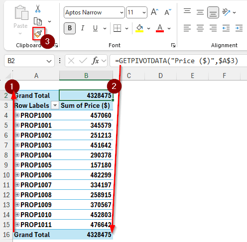
➤ Copy the text Grand Total from the bottom to a row over the pivot table.
➤ Write = in the column next to it and click on the grand total value at the bottom of the sheet so that Excel automatically fills the formula in.
➤ Use Format Painter to copy the grand total format to the new cells.
That was the most convenient way to do that. However, I’m sure you want to know more. In the following, we have the methods explained in detail with a step-by-step guide so that you can understand the techniques properly.
Putting the Grand Total at the Top of the Pivot Table Using a Formula
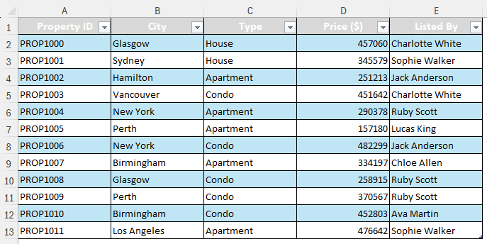
In this dataset, we have some property listings, their prices, the cities where the properties are, the types of properties, and the people who listed the properties.
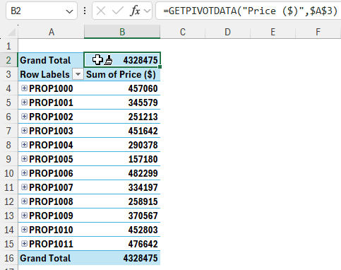
The grand total of the prices is shown at the bottom of the pivot table. While pivot tables allow showing subtotals at the top or bottom, there is no way to show the grand total at the top. Instead of blaming Microsoft, we can get creative and use our own ways to show the grand total at the top. Here is how we do it:
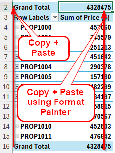
➤ Select the cell that says Grand Total and press Ctrl + C . Go to the top row where you want the grand total to show up, and press Enter.
➤ Right next to that cell, write =
➤ Click on the actual grand total value at the bottom.
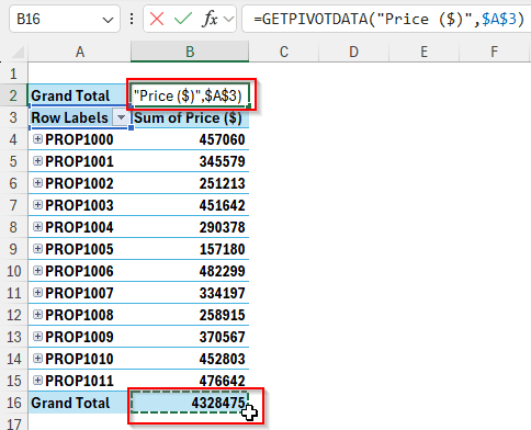
➤ Press Enter.
➤ Right-click on the actual grand total cell (B16 in this case) and click on the Format Painter icon from the context menu.
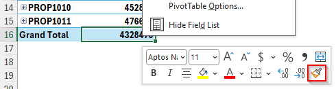
➤ Click on the new grand total cell (B2 in this case) to copy the format.
Showing Grand Total at the Top of the Pivot Table by Modifying Source
While the method we used before is easier, it would not be possible to implement if you don’t have any rows at the top of your pivot table. Fortunately, there is another way to accomplish the task. Follow the steps below:
➤ Go to the source table from which you made the pivot table
➤ In the 2nd cell of the column, right next to the table, write Grand Total.
➤ Upon pressing Enter, Excel would include the column in the table.
➤ Drag your mouse cursor to the bottom to fill the whole column with the same text.
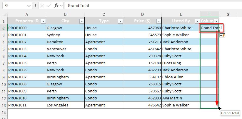
➤ We named the column GT, and the table now looks like this:

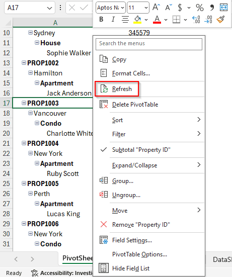
➤ Go back to the pivot table, right-click on the table, and click Refresh from the context menu.
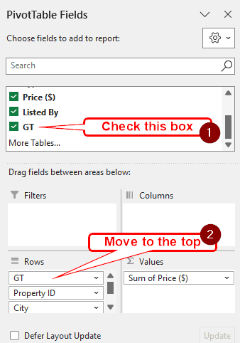
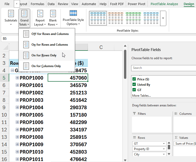
➤ From the PivotTable Fields, check the GT field, and move it to the top of the Rows area.
➤ Now you can disable the grand total at the bottom by going to the Design tab > Grand Totals and selecting On for Rows Only.
Grand Total Based on Two Pivot Tables
Although this method feels kind of like cheating, it works. We are going to use two pivot tables in this method, one for real, one with the grand total only. Follow the steps below:
➤ Select the whole pivot table, and press Ctrl + C to copy it.
➤ Go to the bottom of that table, leave a few rows blank (2-3), and paste the table by pressing Enter.
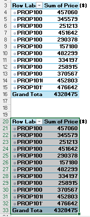
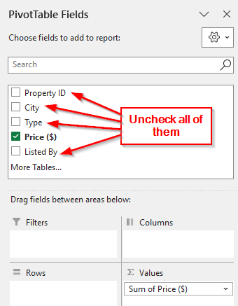
➤ On the second pivot table, uncheck everything from the PivotTable Fields and just keep the numeric field in the Values Here, we are keeping the Price ($) field.
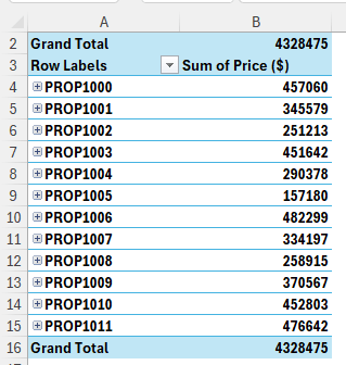
➤ Now the pivot table should look like this:
![]()
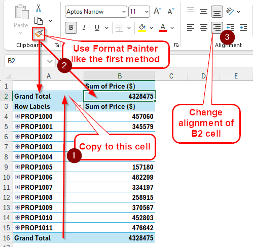
➤ Like we copied and pasted the original table, we are now going to copy and paste this table to the top.
➤ We pasted the Grand Total text at the top and used the Format Painter to copy the cell format in the first method. Do the same thing here.
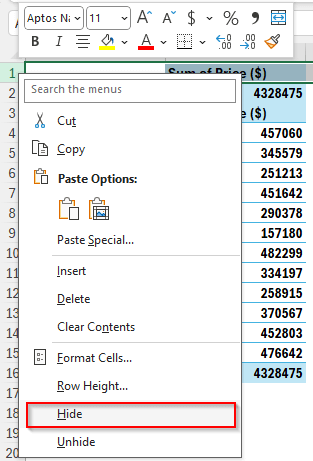
➤ The format of the number cell will not be copied; you would need to copy that from the Grand Total Align the cell to the right from the Alignment group in the Home tab.
➤ We still have the Sum of Price ($) row at the top. We can hide it by right-clicking on the row and selecting Hide.
➤ Now the grand total is at the top like we wanted.
Inserting XLOOKUP Function
We can use a function to find the largest value of the column and use that as our grand total. Here is how to do it:
➤ Write this function at the top of the pivot table:
=XLOOKUP(“Grand Total”,A:A,B:B,,1,-1)
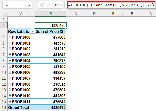
➤ Copy the Grand Total text and the formats for the value using Format Painter, like we did before. The grand total will be what we want:
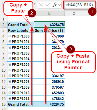
Displaying Grand Total at the Top of the Pivot Table Using MAX Function
This is basically the same as using XLOOKUP; however, the XLOOKUP function is dynamic. That means the previous method can be used no matter how big the pivot table is without editing the function. Using MAX, that would not be the case. Follow the instructions below:
➤ Write this function where you want the grand total to show up:
=MAX(B3:B16)
➤ Do the grand total copy paste and format painter things like before.
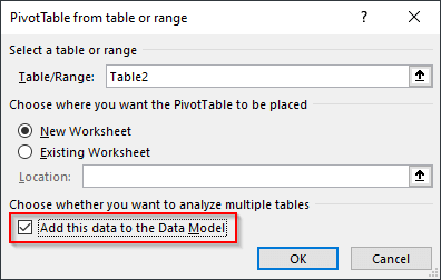
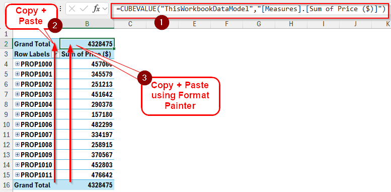
Showing Grand Total at the Top of the Pivot Table Using Data Model
This method requires you to add the pivot table to the data model to make it work. Here are the steps for you to follow:
➤ While creating the pivot table, make sure to tick the box that says Add this data to the Data Model.
➤ Organize and customize your pivot table like you normally do.
➤ Write this function for the grand total:
=CUBEVALUE(“ThisWorkbookDataModel”,”[Measures].[Sum of Price ($)]”)
➤ Don’t forget to copy the Grand Total cell and format the grand total using Format Painter.
Frequently Asked Questions
How do I show totals at the top of a table in Excel?
Insert a row in the table by right-clicking on the row number of the top row and selecting Insert. Then write the formula to get the totals of the columns, and you are done.
How to move subtotal to top in PivotTable?
Select any cell of the pivot table to enable the tabs related to the pivot table. Then, go to the Design tab. From the Layout section, go to Subtotals and click on “Show all Subtotals at Top of Group.”
How to sort grand total in PivotTable?
Right-click on the grand total numbers to open the context menu. From the menu, you can sort using either largest to smallest or smallest to largest.
Why is my PivotTable grand total wrong?
Having the grand total wrong can seem impossible and totally possible for a number of reasons at the same time. If you have a field that is based on other fields, it can mess up the grand total. If you have applied a filter but forgot to turn it off, the grand total can be wrong as well. Missing cells or fields, even a change in the source table, can make the grand total wrong.
How to pivot a table in Excel?
Select the table and go to the Table Design tab. From there, click on Summarize with PivotTable from the Tools section. A new window will pop up. Select whether you want to add the table to the data model or not, where you want to place the pivot table, and press OK.
Wrapping Up
In this article, we have learned the ways you can use pivot table grand total at top in Excel. Don’t forget to practice the methods yourself after downloading the workbook used in this tutorial. Bookmark this site so that you can visit again to learn some more Excel tips, and we will see you in another article.