In a spreadsheet with lots of data, having duplicate cells is not unheard of. Even for genuine reasons, there could be repeating values in a column. For working with those data points, it may be necessary to count the unique values to obtain a proper result. In this article, we will learn how to count unique values excel pivot so that we can accurately perform data analysis.
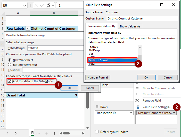
➤ While creating the pivot table, check the box that says Add this data to the Data Model
➤ In the pivot table, set up your rows and values
➤ Click on the desired value field and select Value Field Settings.
➤ Select Distinct Count from the tab on the left, and hit OK
While this was the straightforward method, there are some significant drawbacks to this approach. In this article, we will learn about these issues and also explore an alternative method we can use to avoid those cons. So, stick with us and don’t forget to download the workbook to follow along.
Counting Unique Values in a Pivot Table Using Data Model
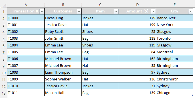
We have a datasheet with some customer transactions in our worksheet today. There are the transaction IDs, the names of the customers, the items they bought, the amount they paid, and the city where they bought it. We want to find the unique customers we have among the names of the customers.
While a pivot table does not directly allow you to count the unique values, the option gets enabled when you use a data model. One disadvantage of this method is that you cannot use this method if your Microsoft Office version is older than 2013. A bigger con of this method is that the unique values are not shown per row; only the grand total of the count can be seen. You will see what I mean in a second. First, follow the steps below:
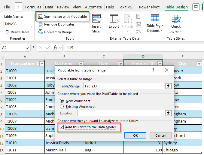
➤ Select any cell of the table to enable the Table Design
➤ Go to that tab. From the Tools group, select Summarize with PivotTable
➤ In the new pivot table, we select Transaction ID and Customer
➤ Move Customer from Rows to Values
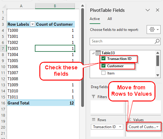
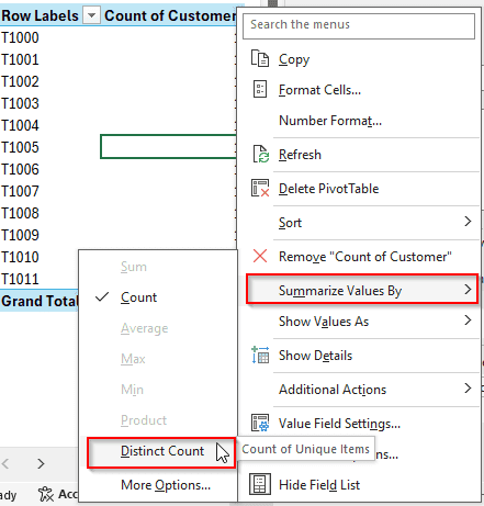
➤ It shows that there are 12 customers. But 12 customers are not unique, we want the unique ones only.
➤ Right-click on any of the cells containing numbers and select Summarize Values By > Distinct Count.
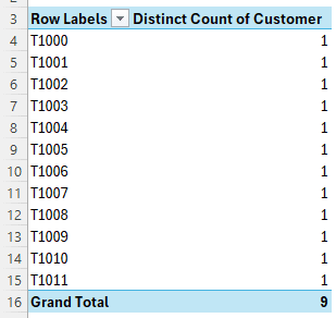
➤ Now the grand total will count the unique values only and leave the repeated values out of the calculation.
Counting Unique Values in a Pivot Table by Adding a Column
If your Microsoft Excel version is older than 2013, or you want to see the repetitive values being counted as 0 in the pivot table, as well as the grand total, you should use this method. This method does not require a data model, but you will need to edit the source table to add a helper column.
➤ Go to your source table and write this formula on the second row (because the first one is the heading) of the column right of the table.
=IF(COUNTIF(B$2:B2, B2) = 1, 1, 0)
➤ Upon pressing Enter, Excel will autofill this formula to the whole column while adding the column to the table as well.
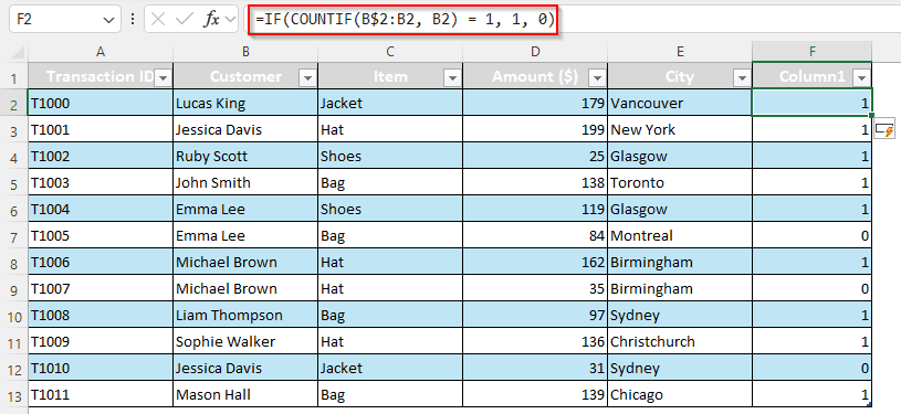
➤ We are renaming Column1 to Unique Customer Count here to make the column name make sense.
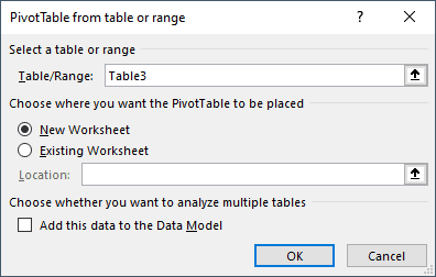
➤ Now, create a pivot table like you usually do; you don’t need to create a data model.
Note:
If you already have a pivot table made from this table, just refresh that table.
➤ Check the Transaction ID and Unique Customer Count boxes from the PivotTable Fields panel.
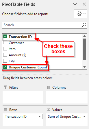
➤ The Transaction ID field should automatically move to the Rows area, and Unique Customer Count should go to the Values area with the name Sum of Unique Customer Count.
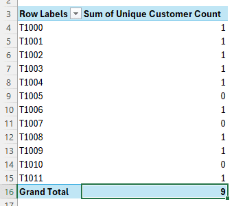
➤ Now, check the pivot table to see the result.
Frequently Asked Questions
Why is distinct count not showing in pivot?
It is either that you are using a very old version of Office, or you have not added the pivot table to the data model while creating the pivot table. You can create another table and add it to the data model for the distinct count to show up.
How do I count only certain values in Excel?
Use the COUNTIF function to count values based on some conditions. The formula is written as follows:
=COUNTIF(range, criteria)
How do I list only unique values in Excel?
Go to the Data tab of Microsoft Excel. From the Sort & Filter group, select Advanced. Select the range and tick the Unique records only option to list the unique values only.
How to refresh pivot table with distinct count?
After selecting the distinct count, the table should refresh automatically. If it does not, make sure that the field is selected from the right panel. Then select any cell of the pivot table, and press Alt + F5 to refresh the pivot table.
How do I show only specific values in Excel?
You can use a filter to show specific values based on a criterion. Filters are available both for regular tables and pivot tables.
Wrapping Up
In this article, we have learned how to count unique values in a pivot table using Excel. We have covered the methods you can use no matter what version of Microsoft Excel is. If you like the tutorial, consider bookmarking the site and visiting us whenever you encounter an issue working with Excel. Download the file used in this tutorial for better clarification, and we will see you in another tutorial.