Google Sheets makes it easy to look up values with the VLOOKUP function. But when you combine it with a drop-down list, you can build dynamic tools like searchable menus, automated forms, and interactive dashboards. This tutorial shows you how to use VLOOKUP with a drop-down to auto-fill data based on user selection.
In this article, you’ll learn how to create a drop-down list, apply the VLOOKUP function, and build a responsive sheet where selecting one value automatically pulls in related information.
Steps to display related information using a drop-down and the VLOOKUP function in Google Sheets:
➤ Select cell D2 where the user will pick a product from a drop-down list
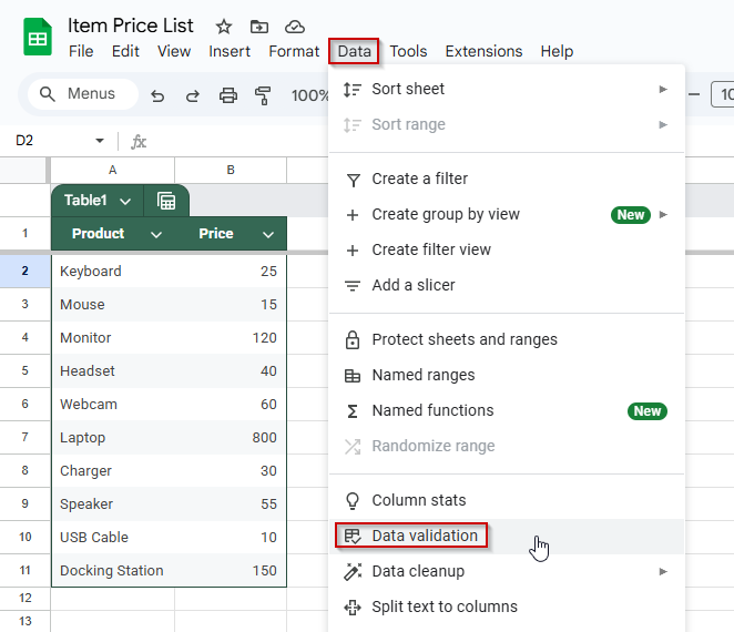
➤ Go to Data >> Data validation to set up the dropdown menu
➤ Set Criteria to: Dropdown (from a range) >> A2:A11, then click Done
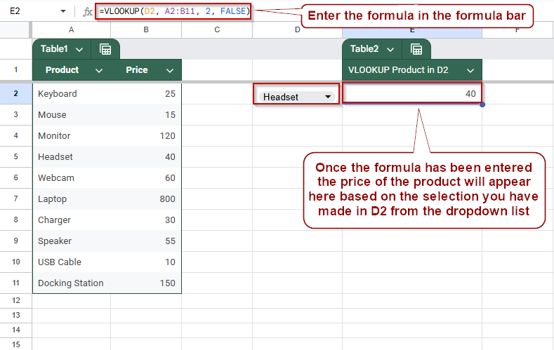
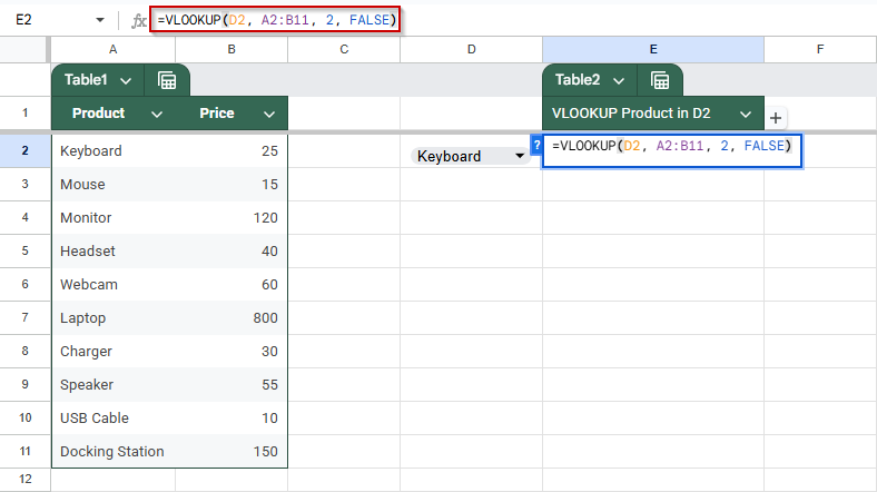
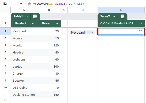
➤ In cell E2, enter the formula: =VLOOKUP(D2, A2:B11, 2, FALSE)
➤ D2: selected product, A2:B11: lookup range, 2: column index for price, FALSE: exact match
➤ The price appears in E2 based on the product selected from the drop-down list
Create a Drop-Down List and Use VLOOKUP
This method demonstrates how to automatically display related information, such as price, based on a user’s selection from a drop-down list. You’ll use the VLOOKUP function to search a data table and return the corresponding value, making your Google Sheet more interactive and efficient.
In this method, you will create a drop-down list of products, and once a product is selected, its price will appear instantly in another cell.
Steps:
➤ Select cell D2 (where the user will choose a product)
➤ Go to Data >> Data validation
➤ Set Criteria to: Dropdown (from a range) >> A2:A11
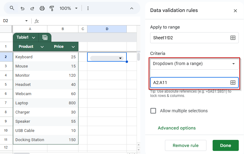
➤ Click Done
➤ In cell E2, enter the following formula:
=VLOOKUP(D2, A2:B11, 2, FALSE)
➧ A2:B11: The data range for lookup
➧ 2: Column number in the range to return (Price is in the second column)
➧ FALSE: Ensures an exact match
➤ Press Enter
Now, whenever you select a product from the drop-down list, the price will appear in E2 automatically.
Setting Up a Dependent Drop-Down With VLOOKUP
This method demonstrates how to create two drop-down lists where the second depends on the first selection. You’ll select a category in the first drop-down, then choose a product from that category in the second drop-down. Finally, the price of the selected product will be displayed using VLOOKUP.
Steps:
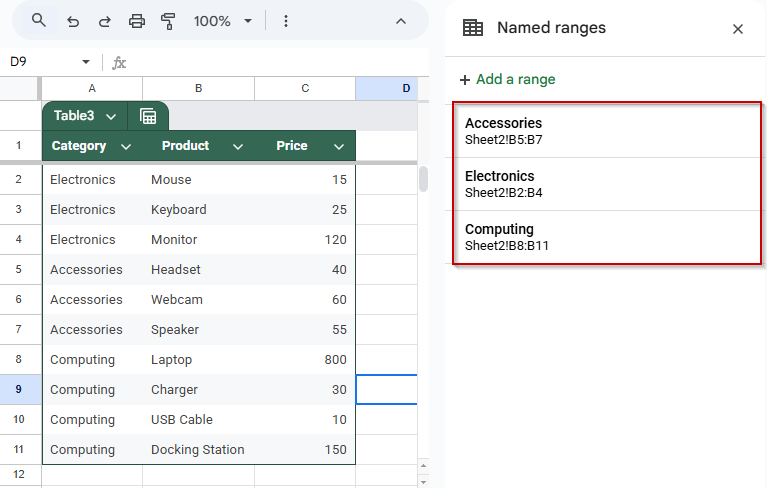
➤ Create named ranges for each category.
➤ Select the group of items you want to assign to a category. Example: Select A2:A4 for products under “Electronics”.
➤ Go to the menu and click Data >> Named ranges.

➤ In the sidebar that appears, type the category name in the field labeled Named range. The name must exactly match the text in the category drop-down (e.g., Electronics).
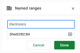
➤ Click Done to save the named range.
➤ Repeat the process for each additional category you have, using their corresponding product lists and exact names.
➤ Select cell F3 (where the user will choose a category)
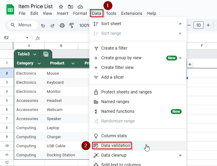
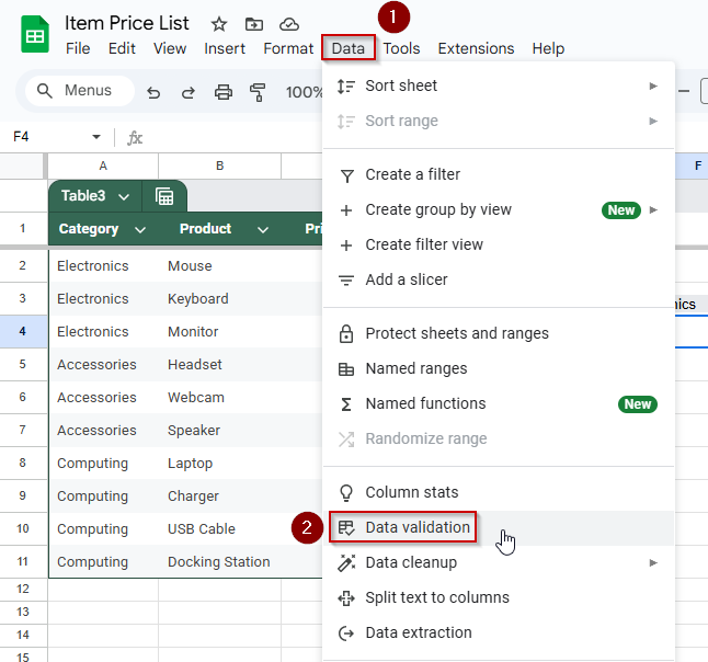
➤ Go to Data >> Data validation
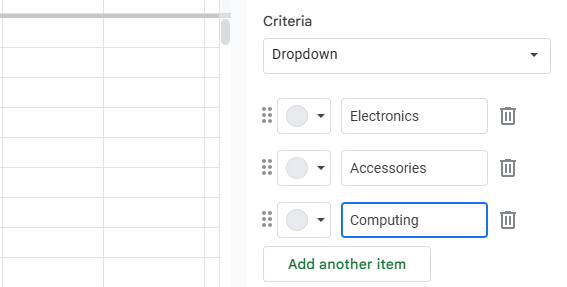
➤ Set Criteria to: Dropdown >> Electronics, Accessories, Computing
➤ Click Done
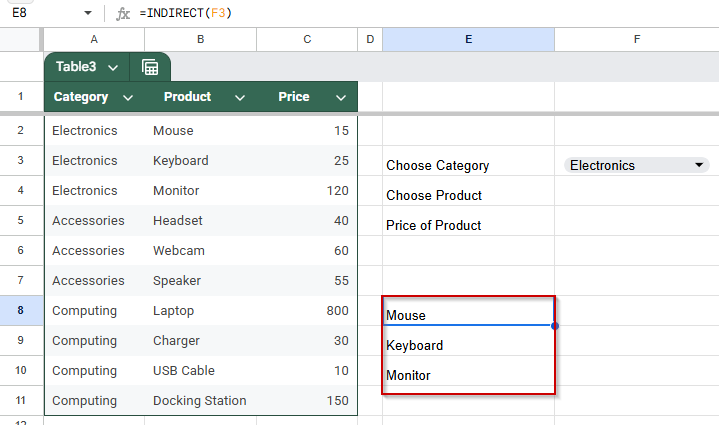
➤ Click on cell E8 and enter this formula to create helper cells:
=INDIRECT(F3)
➤ Select cell F2 (where the user will choose a product based on the category)
➤ Go to Data >> Data validation
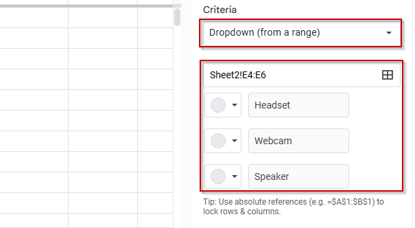
➤ Set Criteria to: Dropdown (from a range) and redirect to the helper cells (E4:E6).
➤ Click Done
➤ In cell G2, enter the following formula:
=VLOOKUP(F4, B2:C11, 2, FALSE)
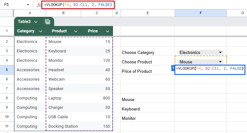
➧ F2: Selected product from the dependent drop-down that changes based on E2
➧ B2:C11: Data range containing products and prices
➧ 2: Column number to return (Price is in the second column)
➧ FALSE: Ensures an exact match
➤ Press Enter
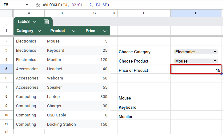
Now, when you select a category in E2, the products list in F2 updates accordingly, and the price for the selected product will appear in G2 automatically.
Frequently Asked Questions
How do I create a dependent drop-down list in Google Sheets?
Create named ranges for each category, use Data Validation for the first drop-down, and apply =INDIRECT(first_dropdown_cell) in the second drop-down’s data validation to make it dynamic.
Why is my VLOOKUP returning #N/A error?
#N/A means no exact match found. Ensure your lookup value matches exactly, the range is correct, and the last parameter in VLOOKUP is set to FALSE for exact matching.
Can I use VLOOKUP with drop-down lists for dynamic pricing?
Yes! Select the product from a drop-down, then use VLOOKUP to fetch the corresponding price dynamically, updating results instantly as you change the selected product.
How do I update a drop-down list when my data changes?
Adjust the range in Data Validation or named ranges accordingly. For dynamic ranges, use functions like OFFSET or ARRAYFORMULA to automatically include new data in your drop-down list.
Wrapping Up
Using dependent drop-down lists combined with VLOOKUP in Google Sheets lets you create dynamic, interactive spreadsheets that simplify data entry and reduce errors. This method is perfect for managing categorized data, like products and prices, without cluttering your sheet. By mastering these tools, you can build smarter dashboards, invoices, or order forms that update automatically based on user selections. Try it out to make your Google Sheets more powerful and user-friendly!