
People who use Google Sheets often need to get more than one value back from a single search key. They might want to see all the products a customer bought or all the students in the department they study in. But the built-in VLOOKUP function only gives you the first match it finds, which isn’t very helpful when there are multiple entries. When a customer might show up more than once in a sales record, for example, a workaround is needed to get all the related values.
You can use FILTER to get all the matching results and TEXTJOIN to put them all in one cell because VLOOKUP only gives you one match.
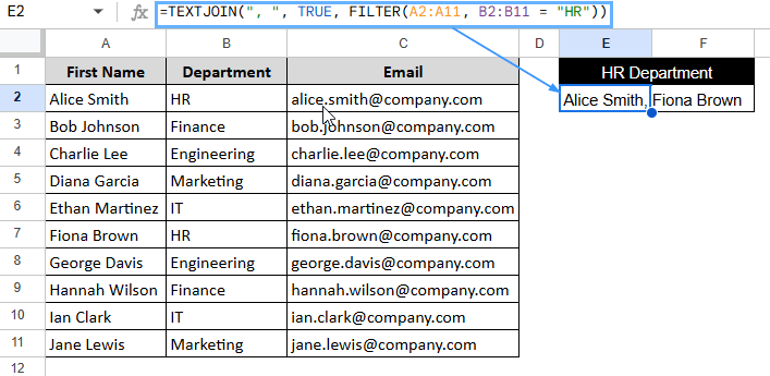
➤ Select E2 cell.
➤ Enter this formula:
=TEXTJOIN(“, “, TRUE, FILTER(A2:A11, B2:B11 = “HR”))
➤ Press Enter to get all employee names from the specified department.
➤ Drag the Fill Handle to get all other data related to column C.
This article will extend beyond the standard “VLOOKUP” and explore alternative methods for retrieving multiple matching values. To meet your needs, we’ll utilize flexible array formulas, custom functions created with Apps Script, and other advanced techniques.
Does VLOOKUP Function Return Multiple Matches in Google Sheets?
The VLOOKUP function in Google Sheets looks for a certain value, known as the search key, in the first column of a defined range. As soon as it finds the first match, it gets a value from a certain column in the same row. VLOOKUP is amazing for single-result lookups because it searches vertically.
VLOOKUP formula syntax:
=VLOOKUP(search-key, range, column-index, [sorted/not-sorted])
VLOOKUP does have a drawback, though: it only gives you the first matching result it finds in the column. If your data has more than one entry for the same key, like more than one employee in the same department, VLOOKUP will only look at the first one.
Alternative to VLOOKUP for Returning Multiple Matches
Google Sheets users often use more flexible functions like FILTER+TEXTJOIN, QUERY, ARRAYFORMULA, INDEX, or even custom solutions made with Apps Script when they need to find more than one match. These tools let you get all the relevant matches, not just the first one.
Using FILTER and TEXTJOIN Functions
VLOOKUP only gives one match; that’s why you can use FILTER to get all the matches and TEXTJOIN to put them all in one cell. This is excellent for summary outputs like names or emails.
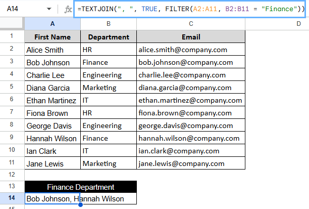
Let’s say we have a dataset of employees that includes their names, email addresses, and the departments they work in. You can use the FILTER and TEXTJOIN Functions to get and show names from a certain department, like “Finance”, in one cell.
Steps:
➤ Select a cell to display the names, e.g., A14.
➤ Enter this formula:
=TEXTJOIN(“, “, TRUE, FILTER(A2:A11, B2:B11 = “Finance”))
➤ Press Enter to get all employee names from the specified department.
Note:
It gives back one cell with all the matches, each separated by a comma. Check that the columns you are referring to don’t have any spaces, or the result might have extra commas.
Using QUERY Function for Advanced Lookups
The QUERY function is very flexible and can return more than one row if a certain condition is met. Those accustomed to SQL-like syntax can also read it more easily. This method works better when you need structured outputs, like having first name, last name, and email all in their columns.
Steps:
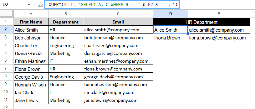
➤ Select an output cell, here E2.
➤ Type the formula:
=QUERY(A2:C, “SELECT A, C WHERE B = ‘” & B2 & “‘”, 1)
➤ Press Enter to return all results vertically.
Note:
This way of exporting full rows of data works very well. QUERY is case-sensitive unless you use extra functions to change that.
Using ARRAYFORMULA with IF for Dynamic Lists
ARRAYFORMULA function is great if you want to match rows and keep the results in the same order as the original rows. It either fills each row with the match or leaves it blank. If your output sheet looks like the original one and you need to line things up, use this.
Steps:
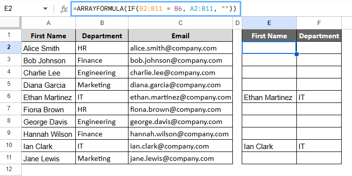
➤ Select an output cell, here E2.
➤ Type the formula:
=ARRAYFORMULA(IF(B2:B11 = B6, A2:B11, “”))
➤ Press Enter to return all results vertically, related to department IT.
Note:
This method keeps the dataset’s row structure. To get a cleaner result, think about wrapping with FILTER to get rid of blank cells.
Using Apps Script to Simulate VLOOKUP for Multiple Matches
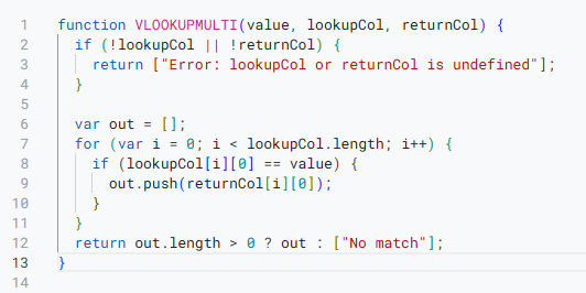
This custom function can help you show results in different rows or cells instead of just one cell with commas separating them. Custom functions let you return values in more than one row, which is helpful for dashboards or data tables where putting all the values in one cell isn’t the best option.
Steps:
➤ Go to Extensions > Apps Script.
➤ Paste the following code:
function VLOOKUPMULTI(value, lookupCol, returnCol) {
if (!lookupCol || !returnCol) {
return ["Error: lookupCol or returnCol is undefined"];
}
var out = [];
for (var i = 0; i < lookupCol.length; i++) {
if (lookupCol[i][0] == value) {
out.push(returnCol[i][0]);
}
}
return out.length > 0 ? out : ["No match"];
}
➤ Now click Run and then Save to drive.
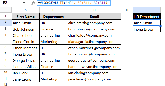
➤ Select an output cell, here E2.
➤ Use the custom function in your sheet:
=VLOOKUPMULTI(“HR”, B2:B11, A2:A11)
➤ Press Enter for the results.
Note:
You only need to permit the custom script once. The script will only work in the Google Sheet where it is saved. If your dataset has thousands of rows, it might slow down a little bit.
Frequently Asked Questions
What is the main difference between FILTER and VLOOKUP?
VLOOKUP only gives you the first match it finds. FILTER can return all matches, which makes it more useful for looking up more than one value.
Can I return values in separate cells instead of one?
Yes. Instead of returning a single cell output, use a custom Apps Script function that returns an array result.
Does the FILTER function support partial matching?
Not directly. You can use REGEXMATCH with FILTER to match parts of a string or a pattern:
=FILTER(ProductRange, REGEXMATCH(CustomerRange, “partial_name”))
Is there a way to get unique values only?
Yes, put your FILTER inside UNIQUE:
=TEXTJOIN(“, “, TRUE, UNIQUE(FILTER(…)))
What if the lookup value doesn’t exist?
The FILTER function will give you a #N/A error. You can use IFERROR to deal with this:
=IFERROR(TEXTJOIN(“, “, TRUE, FILTER(…)), “Not Found”)
Concluding Words
When you need to work with more than one value, VLOOKUP isn’t enough. But Google Sheets has smart alternatives like FILTER+TEXTJOIN, QUERY, ARRAYFORMULA, INDEX, and Apps Script that can get all the matching records. These methods make it easier and more flexible to look at datasets like employee lists.