Blank cells often cause inconsistent results while calculating, transporting data, and applying formulas. With Excel’s Find & Replace tool, you can easily replace all the blank cells in a worksheet with a certain value that you choose.
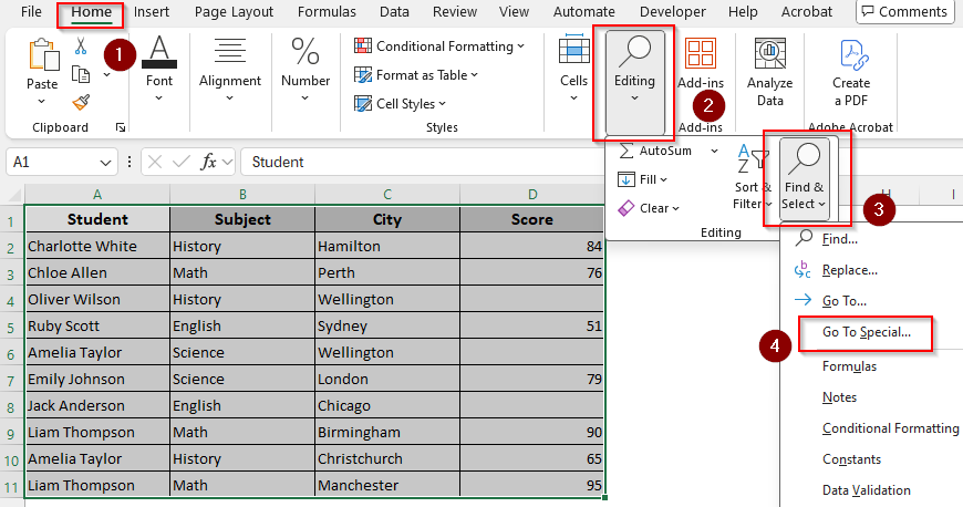
➤ Select the data range with blank cells and go to the Home tab. Click on Editing and choose Find & Select.
➤ From the drop-down menu, select Replace. Or, use the keyboard shortcut CTRL + H .
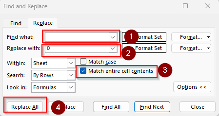
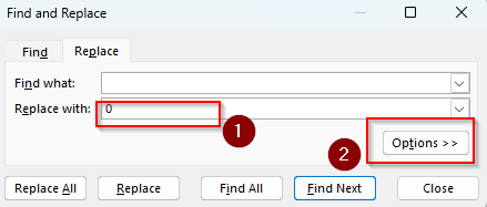
➤ In the Find and Replace dialog box, keep the Find What box blank.
➤ Proceed to the Replace What box and type the value that you want to put in the blank cells.
➤ Go to options and check the Match Entire Cell Contents. Finally, click on Replace All.
Apart from this quick technique, there are other ways to find and replace blank cells with the data you input or values from other cells. In this article, we’ll cover all the possible methods including the power query tool, IF and ISBLANK functions, and VBA coding.
Find Blank Cells and Input Values with the Go To Special Option
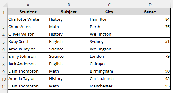
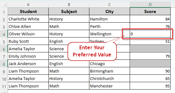
For better visual presentation, we selected a dataset representing a student marksheet for various subjects. In the Score column, the D4, D6, and D8 cells are blank implying that the corresponding students didn’t take the exam. We’ll replace the empty cells with 0.
With this method, you can fill all the blank cells at once with the same value. However, if you have a few blank cells and you want to put different values in each cell, you need to find the cells and fill each cell manually. Here’s how to do it:
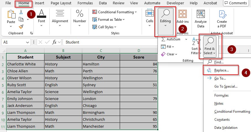
➤ Select your data range and go to the Home tab.
➤ Click on Editing and select Find & Select. From the drop-down menu, choose Go To Special.

➤ Or, use the keyboard shortcut CTRL + G and select Special.
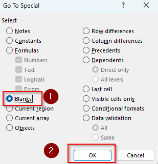
➤ As the Go To Special dialog box appears, click on Blanks and press Ok.
➤ Now, all the empty cells are highlighted. If you want to put different values in each cell, type them manually and press Enter.
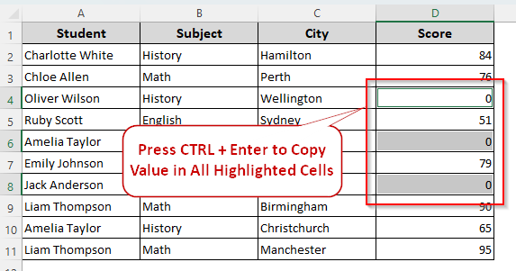
➤ To replace the blank cells with the same value, type the value in any blank cell. Now, press CTRL + ENTER on your keyboard and Excel will replace the same value in all the highlighted empty cells.
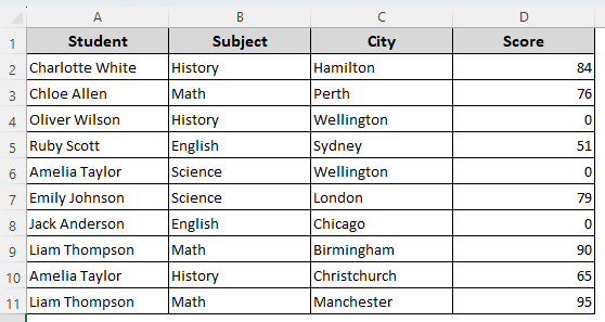
➤ Here’s our final dataset after the replacement:
Fill Empty Cells with the Find and Replace Tool
When you use the Find and Replace tool, it locates all the empty cells and replaces them with the value you put. Let’s get to the steps:
➤ Select your data range and press CTRL + H on your keyboard to use the tool.
➤ Another way is to go to the Home Tab and select Editing from the mini toolbar.
➤ Click on Find & Select and choose Replace from the menu.
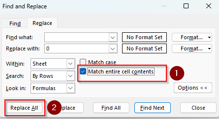
➤ As the Find and Replace dialog box opens, you need to keep the Find What box empty so that Excel locates all the blank cells.
➤ In the Replace What box, enter the value you want to fill the empty cells with.
➤ Click on Options and check the Match Entire Cell Contents box to make sure you only replace entirely blank cells without affecting the ones with hidden values.
➤ Press Replace All, and Excel will notify you of the number of replacements made.
➤ Here’s what our data looks like:

Using the IF and ISBlank Functions to Replace Blank Cells
This method only works when all your empty cells are in a single column. Here, we’ll use the ISBLANK formula to check if a cell is actually blank.
It returns TRUE if it’s blank, and FALSE otherwise. With the IF function, we can replace all the TRUE results with our preferred value.
To apply the functions, follow the steps below:
➤ Create a helper column and type the following formula:
=IF(ISBLANK(D4), “0”, D4)
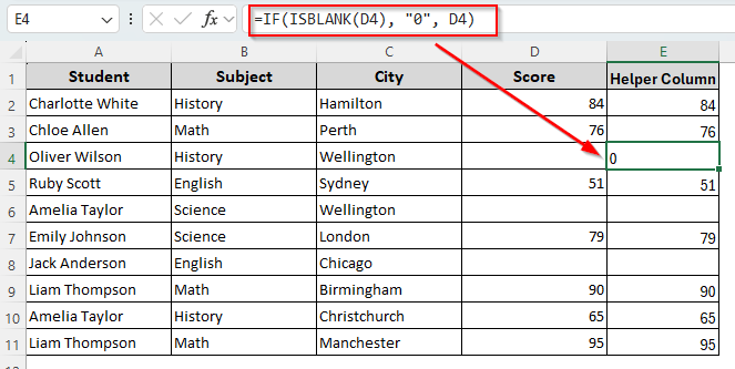
➤ Replace D4 with the neighboring cell reference from the column with empty cells. Instead of 0, put any value you want to fill the blank cells with.
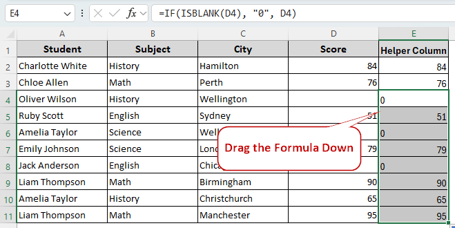
➤ Press Enter and drag the formula down to your last occupied column cell using the fill handle.
➤ You can hide the helper column or copy and paste its materials into the original column.
Note:
If you’re replacing blank cells with numeric data such as 0, it’s better to avoid the quotations (” “) while entering the formula. Otherwise, Excel recognizes the number as a text and puts it in the wrong alignment.
Filling Blank Cells with Data from Cells Above or Below
In this case, you don’t need to put any separate value to fill the empty cells. Instead, you can find those cells and type the cell reference of a neighboring cell to pull data from it. Here are the steps for it:
➤ Select your data range and go to the Home tab. Click on Editing >> Find & Select >> Go To Special.
➤ Choose Blanks from the dialog box options and click Ok.

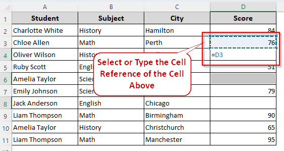
➤ Now, all the blank cells are highlighted. Select the first empty cell and type = in the cell or the formula box.
➤ After that, put the cell reference of the adjacent cell to duplicate its value to the empty cell.
➤ You can also type the reference of the cell above or down to copy the data string from that cell in your chosen blank cell.
➤ For example, our blank cell is D4 and we typed =D3 to copy the content from the cell above.
➤ Press CTRL + ENTER to do the same for each blank cell. Excel will fill the highlighted empty cells with the data from the cell up.

Replacing Blank Cells with Power Query
If you want to automate the blank cell replacing process for future entries, using the Power Query tool will be the best solution. For this, follow the steps given below:
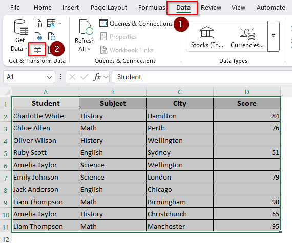
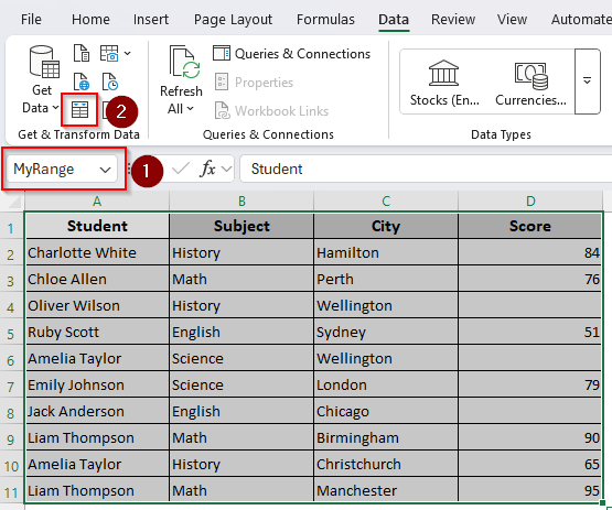
➤ Select your data range and go to the Data tab.
➤ In the Get & Transform Data group, click on the From Table/Range icon.
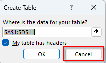
➤ Now, Excel will prompt you to convert your current dataset into an Excel table. You can click Ok if you don’t get bothered by turning the data range into a table.
➤ In case you prefer the current format, press Cancel.
➤ Go to the Name Box and give the data range a name without any spaces. Press Enter and click on the From Table/Range icon again.
➤ As the Power Query Editor opens, go to the Transform tab and select the column you want to change. If there are multiple columns, press CTRL + A to select the entire data range.
➤ Now, click on the arrow beside the Replace Values box on the mini toolbar. Choose Replace Values from the drop-down menu.
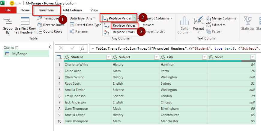
➤ As you can see, Power Query detects empty cells as Null. So, in the Replace Values dialog box, put Null in the Value To Find box.
➤ In the Replace With box, type any value you want. Click Ok.
![]()
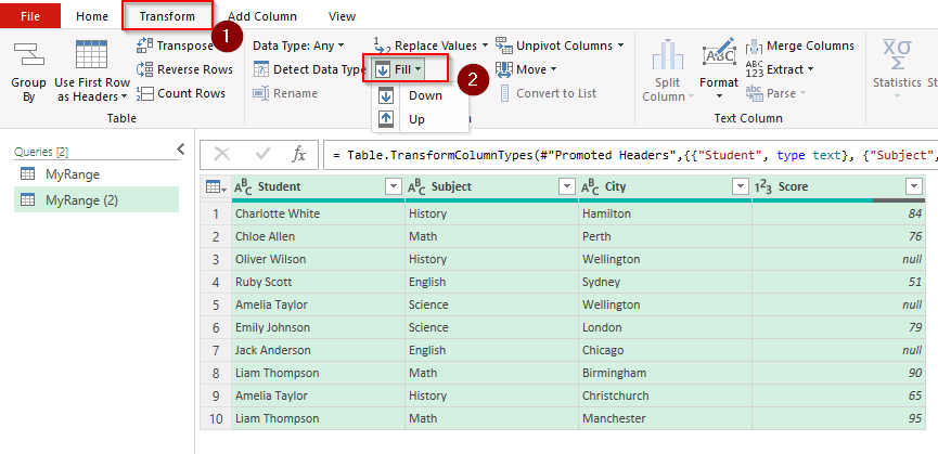
➤ You can also choose to fill the blanks with values from the cell up or down. For this, click on Fill and select Down or Up from the data.
➤ When you’re done replacing the blanks, click on Close & Load.
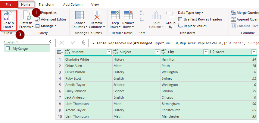
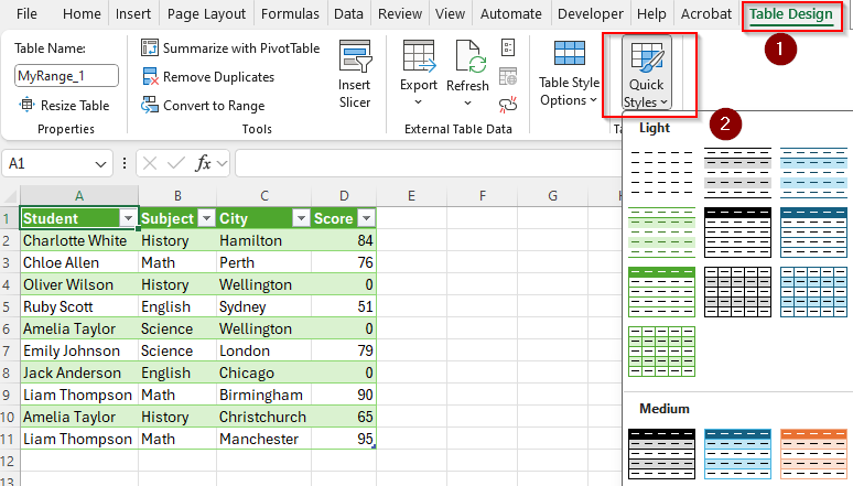
➤ At this point, Excel will rearrange your data with the new values. As Power Query changes the original formatting of your columns, you can open the Table Design tab and choose Quick Styles to change the formatting or completely remove it.
Applying VBA Macro to Replace Blank Cells
Using a macro is a straightforward way to fill empty cells in a complex dataset. To get started, follow the steps given below:
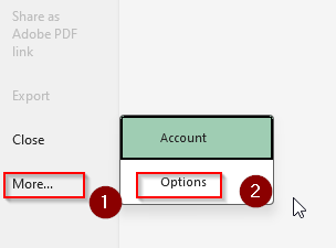
➤ Check if your top ribbon has the Developer tab. If not, go to Files, click on More, and select Options.
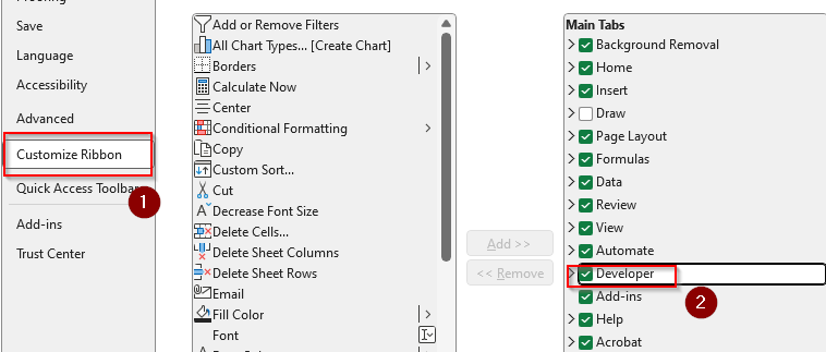
➤ Choose the Customize Ribbon option and check the Developer box. Click Ok.
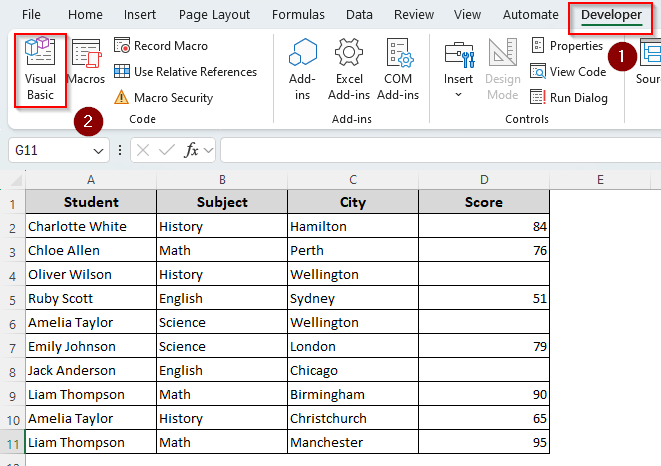
➤ Now, Select your data range. From the Developer tab, choose Visual Basic or use the ALT + F11 shortcut key.
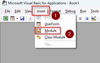
➤ When Excel opens the VBA Editor, click on the Insert tab and select Module.
➤ Copy and paste the following code in the blank box:
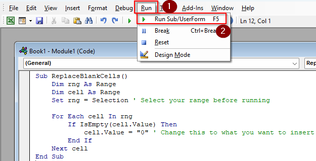
Sub ReplaceBlankCells()
Dim rng As Range
Dim cell As Range
Set rng = Selection ' Select your range before running
For Each cell In rng
If IsEmpty(cell.Value) Then
cell.Value = "YourValue" ' Change this to what you want to insert
End If
Next cell
End Sub
➤ Replace “Your Value” in the 7th line of the code with any other value you prefer to fill the empty cells with.
➤ Press F5 or select Run from the top ribbon. Choose Run Sub/UserForm from the drop-down menu.
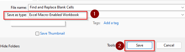
➤ To save the file in the correct format, go to File and click on Save As.
➤ Navigate through your folders to choose your desired location where you want to save the file.
➤ Choose Excel Macro-Enabled Workbook from the Save As Type box and press Save.
➤ Here’s our final dataset:

Frequently Asked Questions
How to remove gaps and make cells blank in Excel?
To remove gaps or spaces from cells and make them blank, create a helper column and type the following formula:
=TRIM(CLEAN(A1))
Replace A1 with the actual cell reference that you want to make blank. Press Enter and drag the formula down to the entire column if there are more cells to clean.
How do you set the #N/A as an empty cell in Excel?
When a formula like VLOOKUP cannot find a referenced value, Excel returns the #N/A error. To prevent it from displaying and showing a blank cell instead, add the IFERROR function to your formula. Here’s an example:
=IFERROR(your_formula, “”)
Put the actual formula instead of your_formula, and Excel will return an empty string if any error occurs.
How do I return a blank cell instead of value?
To return a blank cell instead of 0 or other specific values, type the following formula in a helper column:
=IF(A2=0, “”, A2)
Instead of A2 use your chosen cell reference or a formula. Replace 0 with other specific values that you want to result in a blank.
Wrapping Up
Although Find & Replace is the easiest tool to replace blank cells, it doesn’t work that well with long and complex data sets. Using a formula requires a helper column and Power Query changes the format of the resulting dataset.
However, all these minor changes are easy to fix. Besides, you can use the Go To Special method or apply VBA coding as a quick and accurate solution.