Excel tasks like creating time-based logs, project tracking, scheduling, etc., often require subtracting hours from a specified time. Excel’s TIME function allows you to use the simple Excel subtraction technique to deduct hours from time-formatted cells.
➤ Create a column to enter the final time after the subtraction. In the first cell of the column, insert the following formula:
=C2 – TIME(3,0,0)
➤ This formula subtracts 3 hours from the time entered in cell C2. Change the values according to your dataset.
➤ If you have a different column with hours to deduct, use this formula with your targeted cell references:
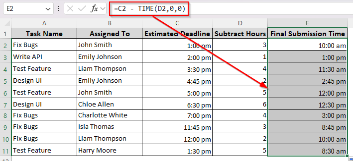
=C2 – TIME(D2,0,0)
➤ Press Enter and drag the formula down to the remaining cells.
Other ways of subtracting hours from time is to use the TEXT, MOD, and IF functions. Read on as this article covers all the different methods of hour deduction in Excel.
Inserting Time Values in the Correct Format
For any time-related calculations in Excel, it’s essential to format the time correctly so that Excel recognizes it. Therefore, before we start, let’s learn how to format your time cells.
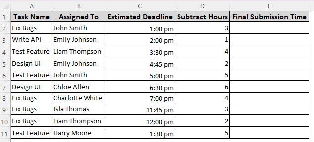
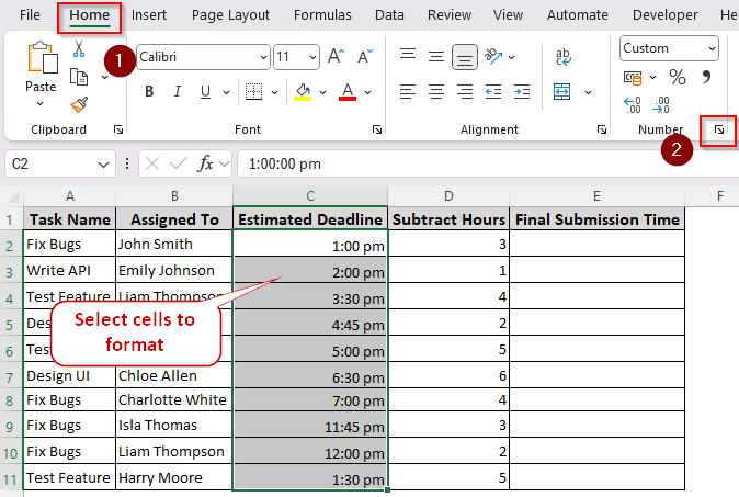
We’ll use a dataset of office task schedules with initial deadlines, deductible hours, and final times in separate columns. Our initial and final time columns are formatted as h:mm AM/PM (1:00 PM).
To format your time column, follow these steps:
➤ Select the cell range, and press CTRL + 1 on your keyboard.
➤ Or, click on the launch icon (downward arrow sign) in the Number group of the Home tab.
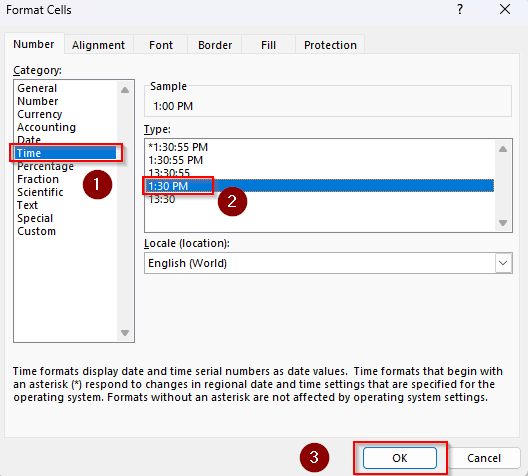
➤ In the Format Cells dialog box, select Time from the Category group and choose any of the following formats:
- h:mm AM/PM (displayed as 1:00 PM)
- hh:mm AM/PM (displayed as 01:00 PM)
- h:mm:ss AM/PM (displayed as 1:00:00 PM)
- hh:mm:ss AM/PM (displayed as 01:00:00 PM)
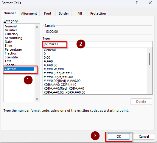
➤ You can also go to Custom and enter a different time format you prefer. For example, if you want to display 1:00 AM as 25:00, go to the Type box and enter [h]:mm as the time format.
Subtracting a Fixed Hour from All Time Cells
Use this method to deduct a specific number of hours from all the initial time cells. We’ll use a simple subtraction formula considering that Excel stores time as fractions of a day. So, 1 hour is 1/24. Here’s how we’ll subtract 3 hours from all the cells of a column:
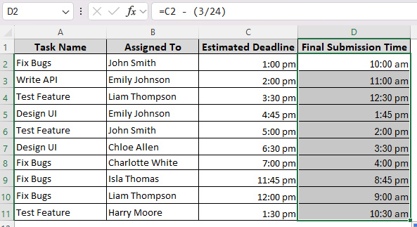
➤ Create a final time column and enter the following formula in its first cell:
=C2 – (3/24)
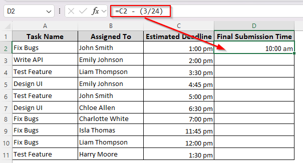
➤ Replace C2 with the appropriate cell reference and 3 with the number of hours you want to deduct.
➤ Click Enter and place your cursor on the bottom right corner of the cell. As the fill handle (tiny arrow sign) appears, drag it down to apply the formula for the following cells.
Subtracting Hours Based on Cell Reference
When you want to deduct different hours from different times, putting them in a separate column is the easy solution. Follow the steps given below to subtract hours using their cell references:
➤ Select the first cell of the final column cell and enter the following formula:
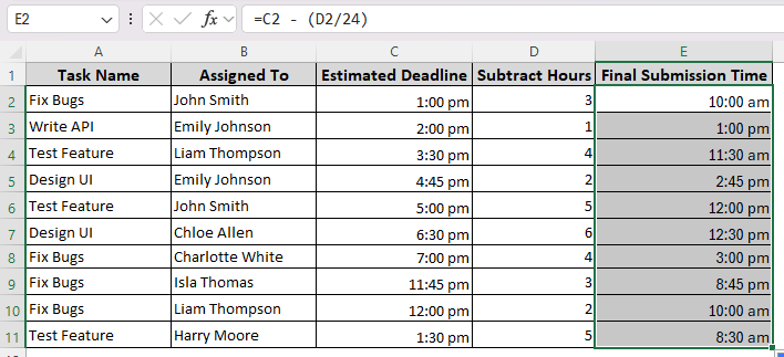
=C2 – (D2/24)
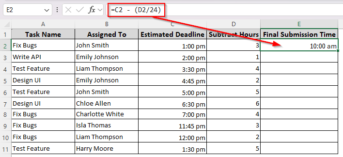
➤ Here, C2 is the cell with the initial time and D2 contains the hours to deduct. Change the cell references according to your dataset.
➤ Click Enter and drag the formula down to get deducted hours in the remaining cells.
Combining the Subtraction Method with the TIME Function
In Excel, the TIME function returns a decimal value of hours, minutes, and seconds. As we’re only working with hours, the remaining values are replaced with zero(0) in the subtraction formula. Here’s how:
➤ Choose a cell from the final time column and insert any of the following formulas:
For Fixed Hours
=C2 – TIME(3,0,0)
For Cell References with Different Hours
=C2 – TIME(D2,0,0)
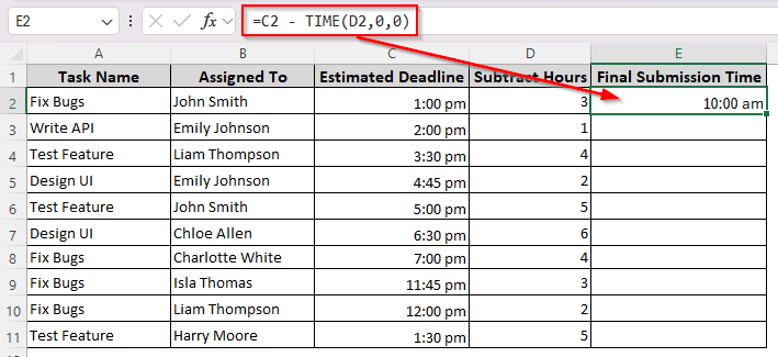
➤ Replace C2 and D2 based on the initial time and subtract hour cells of your dataset.
➤ Press Enter and drag the fill handle down to apply the formula to the rest of the cells.

Deduct Hours and Specify Time Format with the TEXT Function
While the TEXT function is useful for converting time into a readable format, you can’t format the resulting time as an Excel-recognized time format. Therefore, you can’t perform any time calculations later on with the final time. Keeping this in mind, let’s proceed to the steps:
➤ In a final time column cell, enter any of the following formulas:
For Fixed Hours
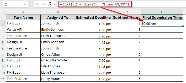
=TEXT(C2 – TIME(3, 0, 0), “h:mm AM/PM”)
For Cell References with Different Hours
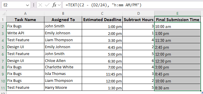
=TEXT(C2 – (D2/24), “h:mm AM/PM”)
➤ Instead of C2 and D2, use the appropriate cell coordinations containing your initial time and deductible hours.
➤ Insert the formula by clicking Enter and drag the formula down to the end of the time cells using the fill handle.
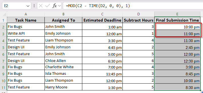
Use the MOD Function for Times Crossing Midnight
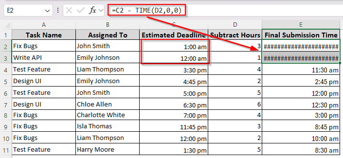
If the subtraction causes the final time to cross midnight, the previous formulas return a negative value, hash symbols(######), or value error(#VALUE). It happens when we only display time, but not dates.
To demonstrate how the function works, we’ve changed the first two cells of our dataset so that the final time gets past midnight. Here’s what happens when we apply the TIME function and subtraction formula to the cells:
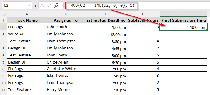
To handle this, we’ll use the MOD function in the following way:
➤ In the first cell of the final time column, type any of the following formulas:
For Fixed Hours
=MOD(C2 – (3/24), 1)
Or,
=MOD(C2 – TIME(3, 0 , 0), 1)
For Cell References with Different Hours
=MOD(C2 – (D2/24), 1)
Or,
=MOD(C2 – TIME(D2, 0 , 0), 1)
➤ Adjust the cell references and hours based on your dataset times.
➤ Click Enter and drag the formula down to fill the remaining cells.
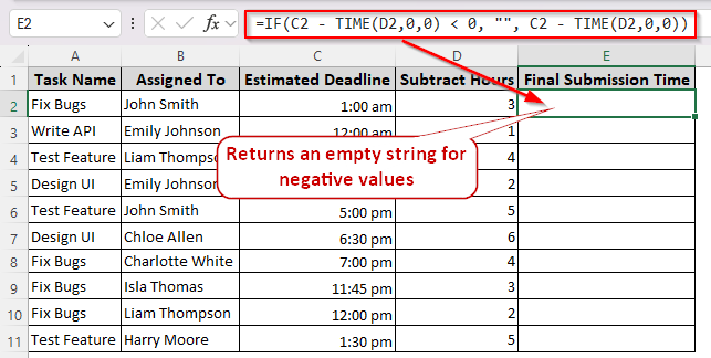
Handling Negative Subtraction Results with the IF Function
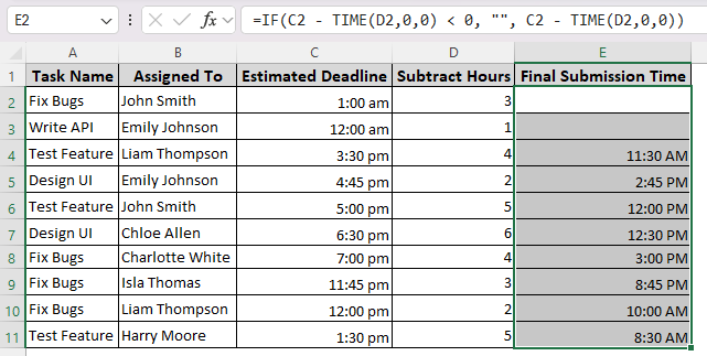
Another way to handle negative values resulting from the subtraction is to use the IF function. After changing the values for the first two cells as described in the previous method, we’ll apply a formula that returns an empty string for negative time values. Below is the process of using it:
➤ Choose a cell from the result time column and insert either of the following formulas:
For Fixed Hours
=IF(C2 – TIME(3,0,0) < 0, “”, C2 – TIME(3,0,0))
For Cell References with Different Hours
=IF(C2 – TIME(D2,0,0) < 0, “”, C2 – TIME(D2,0,0))
➤ Replace the cell references and deducting hours with the actual values of your dataset.
➤ Click Enter and use the fill handle to apply the formula to more cells. With this formula, Excel returns empty strings for times past midnight.
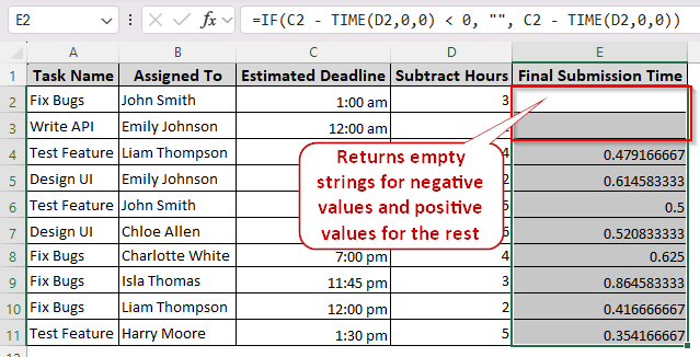
➤ As you can see, Excel displays the deducted times as numbers. To change the format, click on the launch icon on the Number group.
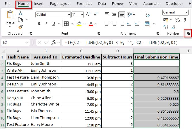
➤ Select Time from the Category group and choose your preferred time format. Finally, click Ok.
Frequently Asked Questions
How to show negative time in Excel?
To show negative time, you need to apply Excel’s 1904 date system. For this, go to File >> More >> Options >> Advanced. Scroll down to locate the When Calculating This Workbook group. Check the Use 1904 Date System box and press Ok.
How do I convert deducted time to integer hours in Excel?
Adding an INT function to your time formula will display hours rounded as integers. For example, to deduct 3 hours from cell C2 and only display the whole numbers in hours, enter the following formula in a cell:
=INT((C2 – TIME(3,0,0)) * 24))
How to separate hours from time in Excel?
Using the HOUR() function will extract the hour part of the time. Enter either of the following formulas in an appropriate cell:
=HOUR(12:45:30) or, =HOUR(D2)
Here, D2 is the cell reference containing the time in hh:mm:ss format. In both cases, the formula returns 12.
Wrapping Up
Subtracting hours from time is a straightforward way as long as you follow the correct format. Although a simple subtraction usually works, you might face errors or get results as numbers.
If the formula returns hash symbols(######), adjust your cell’s width and format the cell with the correct time format. Similarly, format the resulting numbers to time if a formula returns numbers.