When you transfer data from a different system to Excel, you might find carriage returns putting each text in a different line. As they often interfere with data processing, formatting, and analysis, you need to eliminate them using quick and easy methods like applying a formula.
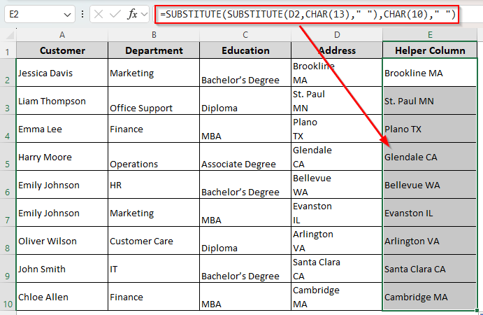
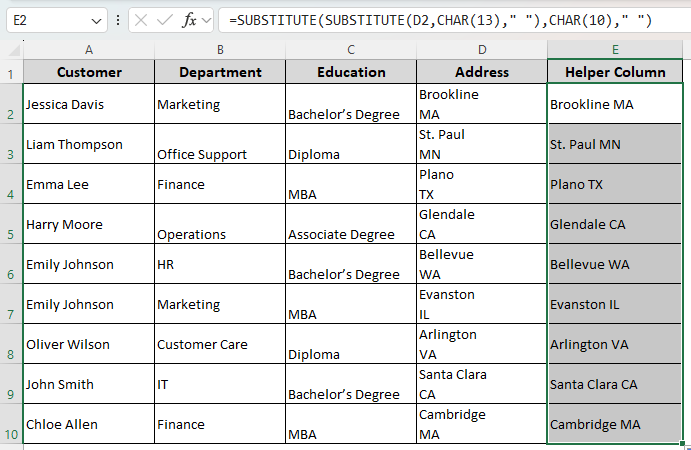
➤ Create a helper column and enter the following formula in a cell adjacent to your first data string:
=SUBSTITUTE(SUBSTITUTE(D2,CHAR(13),” “),CHAR(10),” “)
➤ Replace D2 with the cell reference containing the text string with carriage return.
➤ This formula replaces carriage returns with spaces. You can also put a comma between the quotation marks (“,”) to separate the texts.
➤ Press Enter and apply the formula to the remaining cells using the fill handle.
Apart from this quick method, you can use the Flash Fill feature, Find & Replace tool, TRIM & CLEAN functions, or VBA coding. This article covers all the possible ways of removing carriage returns in Excel.
Using the Flash Fill Feature to Remove Carriage Returns
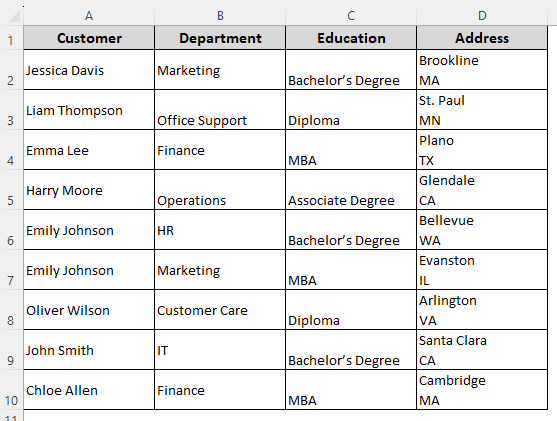
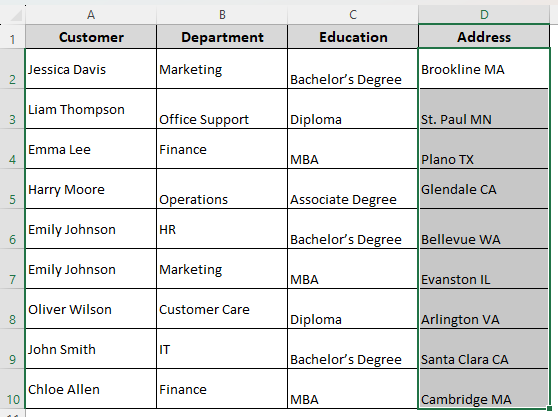
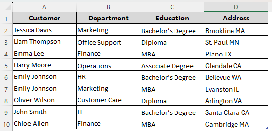
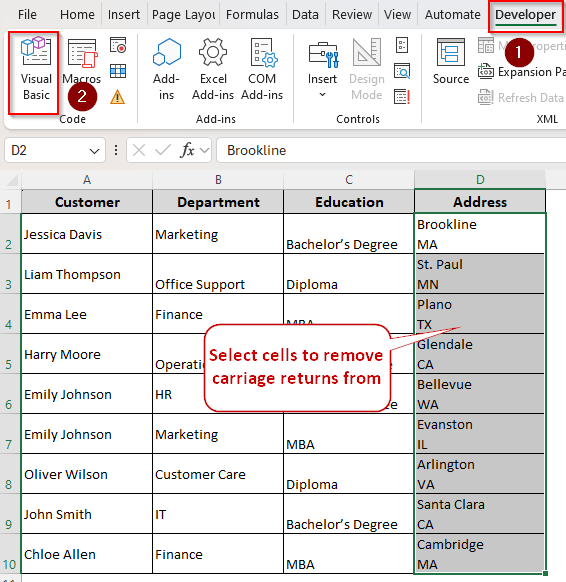
In our dataset, we have columns for employee info including their name, department, educational qualification, and short address. In the address column (column D), all the cells have carriage returns or line breaks.
Our target is to remove them and replace them with a single space. You can use other delimiters such as a comma, dash, semicolon, etc.
For a small dataset, using the Flash Fill feature is the easiest way to eliminate carriage returns. It helps Excel to recognize patterns from the given examples and apply them to the selected cells. Let’s get to the steps:
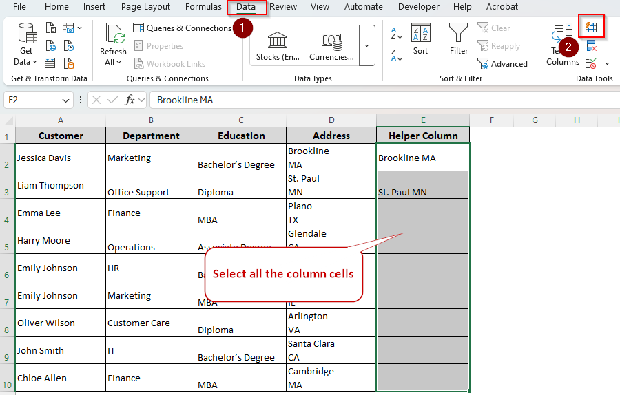
➤ Create a helper column and manually type the corrected texts without carriage returns in the first two cells as shown below:
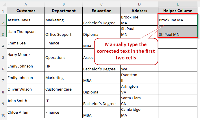
➤ Now, select all the column cells adjacent to the original text strings and press CTRL + E .
➤ Or, you can go to the Data tab and click on the Flash Fill icon in the Data Tools group.
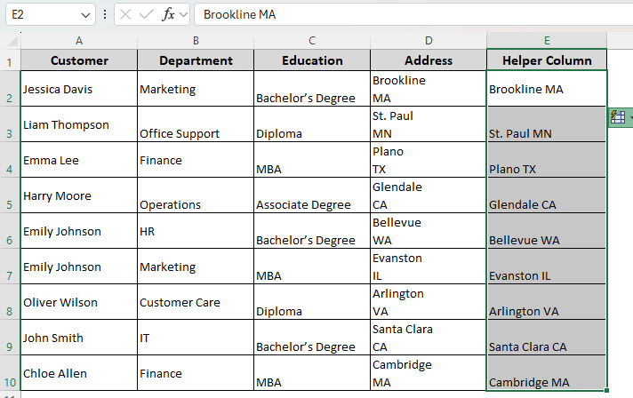
➤ Now, Excel will fill the selected cells with the corrected data. In case it misses, select another cell and repeat the process.
Removing Carriage Returns with the Find & Replace Tool
To quickly eliminate carriage returns, you can use the Find & Replace tool. All you need to do is guide it to locate the carriage returns and replace them with your preferred characters. Here’s how:
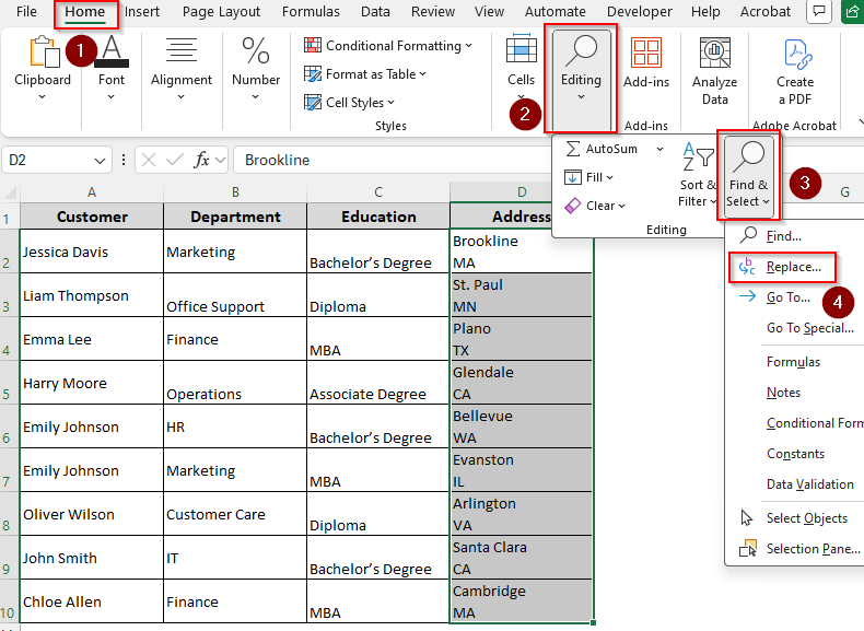
➤ Use the keyboard shortcut CTRL + H or go to the Home tab and click on the Editing group. Select Find & Select and click on Replace.
➤ In the Find and Replace dialog box, type CTRL + J in the Find What field. It’s the keyboard shortcut for carriage returns or line breaks. You might notice a tiny dot (.) in the box.
➤ Choose your preferred delimiter and enter it in the Replace With field. We’ll only enter a space for our dataset.
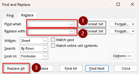
➤ Click Replace All and Excel will replace all the carriage returns with your chosen character.
Creating a Formula with the TRIM and CLEAN Functions
In Excel, the CLEAN function eliminates all the non-printable characters including carriage returns. On the other hand, the TRIM function removes all the extra spaces from the dataset and keeps only single spaces. So, we’ll combine the two functions in the following way:
➤ In a helper column cell, insert the following formula:
=TRIM(CLEAN(D2))
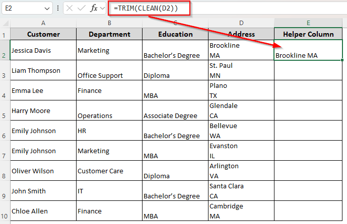
➤ Replace D2 with the cell reference containing the text with carriage returns.
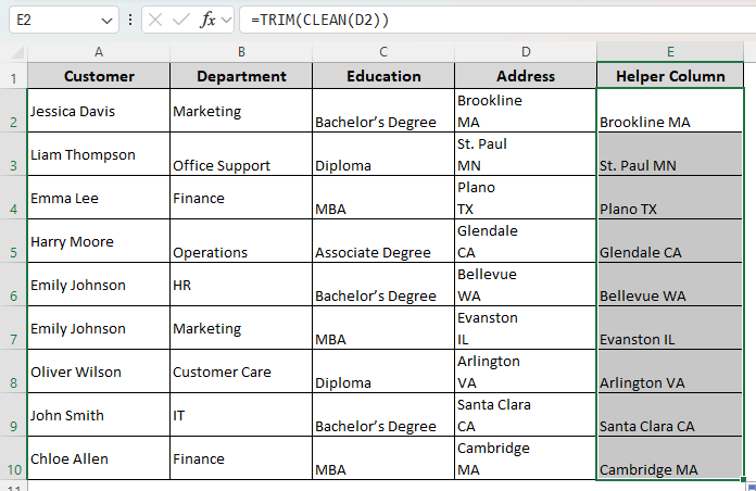
➤ Click Enter and use the fill handle (tiny + sign on a cell’s bottom corner) to apply the formula to the remaining cells.
Eliminating Carriage Returns with the SUBSTITUTE Function
Using the SUBSTITUTE function allows you to replace carriage returns with your specified characters. In Excel, CHAR(13) represents the carriage return character and CHAR(10) represents the line feed character.
Therefore, the following method will eliminate both carriage returns and line breaks. Below are the steps:
➤ Choose a helper column cell and enter the following formula:
=SUBSTITUTE(SUBSTITUTE(D2,CHAR(13),” “),CHAR(10),” “)
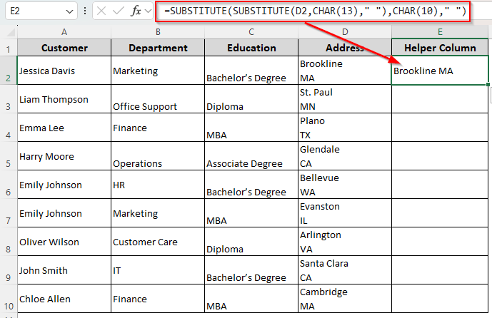
➤ Instead of D2, use the appropriate cell reference containing the carriage returns. You can also place a delimiter within the quotation marks (such as “,”).
➤ Click Enter and drag the formula down to the last cell using the fill handle.
Using Text to Columns Wizard to Separate Texts Based on Carriage Return
With the Text to Columns feature, you can remove carriage returns and put the separated text in two different columns. However, it’s not effective to just remove the carriage returns and directly join the data in the same column. Let’s get to the steps:
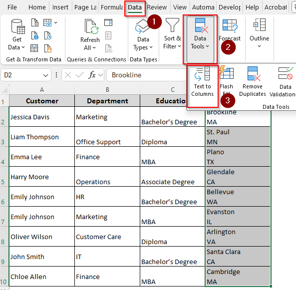
➤ Go to the Data tab and click on Text to Columns.
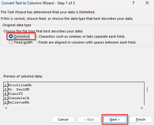
➤ As the Step 1 of the Text to Columns Wizard box appears, choose Delimited, and click Next.
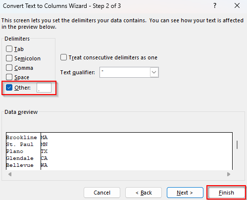
➤ In Step 2, uncheck all the given options and select Other. Press CTRL + J in the box. Click Finish.
➤ Now, Excel will create separate columns for each carriage return. Here’s what our dataset look like after organizing:

Dynamically Remove of Carriage Returns with the Power Query Tool
Replacing carriage returns with the Power Query tool is similar to using the Find & Replace tool. However, the changes made within this tool are dynamic, so they apply to your future entries in the same workbook. If you prefer this, follow the steps given below:
➤ Select your data range and go to the Data tab. Navigate to the Get & Transform Data group and click on the From Table/Range icon.

➤ Click Ok if prompted to create a table.
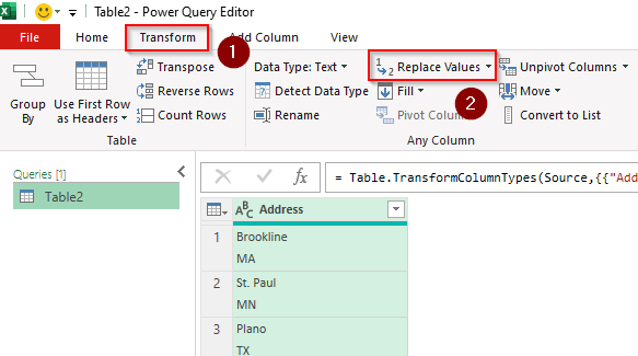
➤ As the Power Query Editor opens, click on the Transform tab and select Replace Values.
➤ In the Value to Find field, press CTRL + J to find all the line breaks. Instead of this, you can type #(cr) for carriage returns or #(lf) for line feeds.
➤ Keep the Replace With field empty or enter your preferred delimiter.

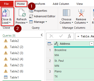
➤ Press Ok. Once the changes are made, click on Close & Load.
➤ Copy and paste the data over the original column and make the necessary changes to the formatting. Here’s our final result:
Customizing a VBA Macro to Eliminate Carriage Returns
Coding with the VBA editor allows you to effectively remove carriage returns from a complex dataset. Here’s how to proceed with it:
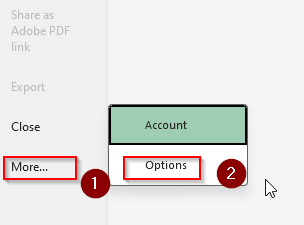
➤ To add the Developer tab on the top ribbon, go to File >> More >> Options.
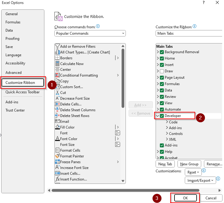
➤ Select Customize Ribbon from the side column and check the box beside the Developer option. Press Ok.
➤ Now, click on the Developer tab and go to Visual Basic.
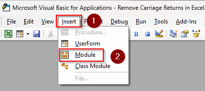
➤ In the VBA Editor, click on the Insert tab and select Module.
➤ When the new module box appears, copy and paste the following code in it:
Sub RemoveCarriageReturnsWithDelimiter()
Dim Rng As Range
Dim Cell As Range
Dim Delimiter As String
' Prompt the user to select a range
On Error Resume Next ' Handle case where user cancels selection
Set Rng = Application.InputBox(Prompt:="Please select the range of cells to clean.", Type:=8)
On Error GoTo 0 ' Reset error handling
' Check if a range was selected
If Rng Is Nothing Then
MsgBox "No range selected. Operation cancelled.", vbInformation
Exit Sub
End If
' Prompt the user for the delimiter
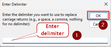
Delimiter = InputBox("Enter the delimiter you want to use to replace carriage returns (e.g., a space, a comma, nothing for no delimiter):", "Enter Delimiter")
' Check if the user cancelled the delimiter input
If Delimiter = "" And Len(Delimiter) = 0 Then ' Check for empty string and cancelled input
If MsgBox("You did not enter a delimiter. Do you want to remove carriage returns without replacement?", vbYesNo + vbQuestion, "No Delimiter Entered") = vbNo Then
MsgBox "Operation cancelled.", vbInformation
Exit Sub
End If
End If
' Loop through each cell in the selected range
Application.ScreenUpdating = False ' Turn off screen updating for performance
For Each Cell In Rng.Cells
' Replace carriage returns (Chr(13)) and line feeds (Chr(10)) with the specified delimiter
' Chr(13) is a carriage return
' Chr(10) is a line feed
Cell.Value = Replace(Cell.Value, Chr(13), Delimiter)
Cell.Value = Replace(Cell.Value, Chr(10), Delimiter)
Next Cell
Application.ScreenUpdating = True ' Turn screen updating back on
MsgBox "Carriage returns removed from selected data using '" & Delimiter & "' as the delimiter.", vbInformation
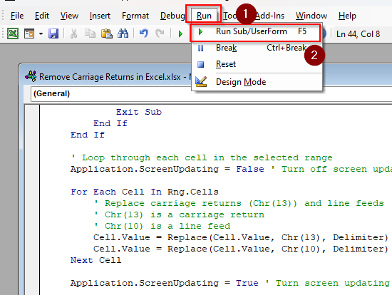
End Sub➤ Press F5 or go to the Run tab and click on Run Sub/UserForm.
➤ When prompted, select your data range from the Excel tab and enter a delimiter.
➤ Go back to the Excel tab to review the changes.

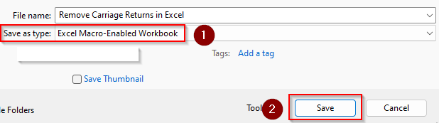
➤ To save the file, click on the File tab, select Save As, and choose a location.
➤ Click on the arrow beside the Save as Type box, select Excel Macro-Enabled Workbook, and press Save.
Frequently Asked Questions
How do I fix the row height after removing carriage returns?
If Excel doesn’t automatically fix the row height after removing the carriage returns, select the rows and go to the Home tab. In the Alignment group, uncheck the Wrap Text box. With the rows still selected, go to the Cells group, click Format, and choose AutoFit Row Height.
How do you paste from Excel cell without carriage returns?
When copying from an Excel cell itself, double-click the cell you want to copy from, or select it and press F2 to put it in Edit mode. Select all the text within the cell by pressing CTRL + A . Copy the selected text with CTRL + C . Go to your destination cell and paste with CTRL + V . This way, you’re copying only the raw text content without the formatting.
How to remove only the last carriage return in a cell?
To remove only the last carriage return from a cell, create a helper column and insert the following formula:
=SUBSTITUTE(D2,CHAR(10),””,LEN(D2)-LEN(SUBSTITUTE(D2,CHAR(10),””)))
Change the cell reference D2 based on your dataset and add a delimiter between the first quotation marks if you prefer.
Concluding Words
As we’ve learned, multiple Excel features and formulas allow you to remove carriage returns and join the texts. While using the SUBSTITUTE function, you can specify a delimiter to separate the joint texts.
For smaller datasets, use the Flash Fill feature for a quick solution to the problem. However, using a formula or VBA macro is recommended for precise removal and better customization.