When investing in a business project, the cash flow is usually not the same over the years. In order to justify an investment, we need to calculate the present value of the future cash flow. In this article, we will learn how to calculate present value in excel with different payments.
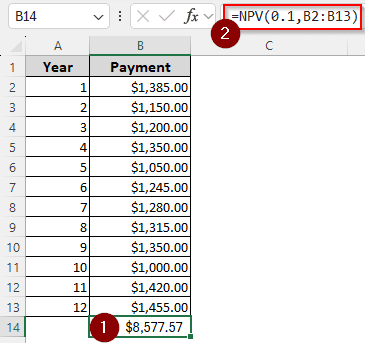
➤ Write this formula where you want the sum of the present value with different payments: =NPV(0.1,B2:B13)
➤ Replace 0.1 with the discount rate and B2:B13 with the range of cash flow.
➤ Press Enter.
That method provides the sum of present value with a static discount rate. But, as you have different payments, you might have different discount rates as well. In this article, we will show how to calculate using both constant and variable discount rates, and how to calculate the present values of each individual payment. Therefore, read the whole tutorial and follow along using our workbook, which is available to download for free.
What is Present Value of Money?
According to the time value of money, the worth of cash decreases over time due to various reasons. Receiving 10 dollars today is worth more than receiving 10 dollars a month later. The value of money declines because of inflation, investment, risks, etc.
When you convert the value of money you will receive in the future to today’s value, you get the present value of money. For example, if you receive 100 dollars in the next year, and the discount rate is 10%, that 100 dollars is worth 90.91 dollars today. The discount rate is calculated using the bank interest rate, inflation rate, investment return, etc.
Calculating Present Value with Different Payments Using NPV
Although the NPV (Net Present Value) function is typically used for investment returns, we can also use it for our purpose. This function calculates the present value regardless of the dates and provides the sum of the amount as the result.
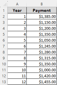
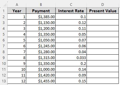
To illustrate the usage of this function, we have a dataset with 12 years of payment, and the payment is not constant. The discount rate is the same for all of them, which is 10%. We are going to use the NPV formula for this calculation. Here is what you need to do:
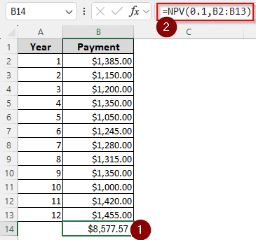
➤ In the B14 cell, we want to see the present value. Therefore, we write the following formula in that cell:
=NPV(0.1,B2:B13)
➤ Press Enter to see the result.
Determining Present Value with Variable Rate of Return Using PV
In the previous formula, the rate of return (or the discount rate) was 10% for all the payments. However, if you have a long period of time, such as 12 years, the rate might change. This time, we will use different rates to do the job and use the PV function in Excel. Follow the steps below:
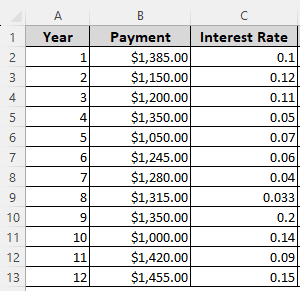
➤ Here, we will calculate present values first and then determine the sum of the values. Therefore, create a heading called “Present Value” in the D column.
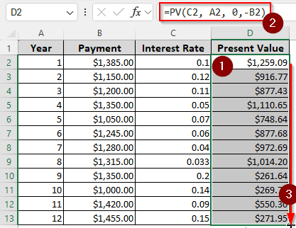
➤ In D2 cell, write this formula:
=PV(C2, A2, 0, -B2)
➤ Press Enter and go to the bottom-right corner of the D2 cell to find a plus (+) sign. Drag that sign to the D13 cell to autofill the formula and do the calculation for all the rows.
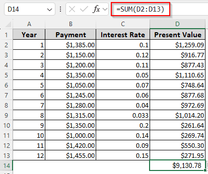
➤ Now, in D14 cell, write this formula to sum up the values:
=SUM(D2:D13)
➤ Press Enter.
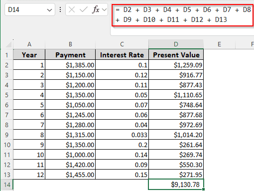
Finding the Present Value with Different Payments Manually
In both of the formulas used before, we made use of functions provided by Microsoft Excel. This time, we will be doing the calculations manually, including the summation at the end. We will be using the same dataset we used in the previous method for this calculation. Here is the process of calculation:
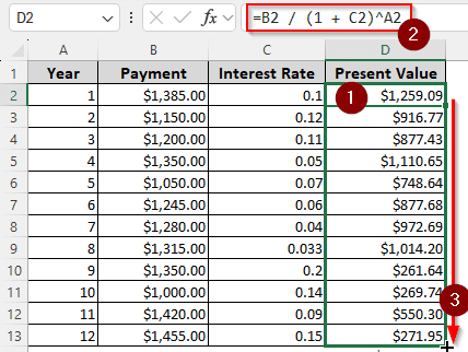
➤ In D2 cell, write this formula:
=B2 / (1 + C2)^A2
➤ Autofill other rows by dragging your mouse.
➤ In D14 cell, calculate the sum of the whole column using the following formula:
= D2 + D3 + D4 + D5 + D6 + D7 + D8 + D9 + D10 + D11 + D12 + D13
Frequently Asked Questions
How do you calculate FV with different payments?
You can use the following function to do so:
=FV(0.1, A1, 0, B1)
Replace 0.1 with the interest rate, A1 with the payment period, and B1 with the value.
How to find the present value of each payment?
Here is the formula to calculate the present value of each payment:
=A1/((1+0.1)^B1)
You need to replace A1 with the future value of the payment, 0.1 with the discount rate, and B1 with the year count (Don’t put the actual year, put the count like 1/2/3)
What is the difference between NPV and PV in Excel?
The NPV function calculates the net present value, which means it sums up all the present values in one cell. The PV function gives the present value of a single input. NPV can make use of a large data range as an input, while PV cannot.
How do you calculate interest rate with different payments?
If you need to make payments multiple times in a year, you have to divide the yearly interest rate by the number of times you will make the payment. The formula can be written like this in Excel:
=0.1/12
Here, we assume that you have a 10% interest rate (written as 0.1), and you need to make a monthly payment, so we are dividing by 12.
How do you calculate future value with different interest rates?
Format your formula like this:
=A1*((1+0.1)^B1)
Change A1 to the present value, 0.1 with your interest rate, and B1 with the year count. Now use this formula over all of the payments while using different interest rates. Sum up the values at the end if you want.
Wrapping Up
In this article, we have learned how to calculate present value in Excel with different payments. We hope that you have been able to learn all the methods we have used in this article. Remember to leave your feedback below; we love to read your comments.