Consolidating data from multiple columns into a single, organized list is a common task when working with Excel. Whether you’re combining sales figures, survey responses, or inventory data spread across several columns, Excel provides various effective methods to help you merge this data perfectly. Knowing how to consolidate data efficiently can save you hours and reduce errors.
In this article, you’ll learn all the best ways to consolidate data from multiple columns in Excel. We’ll cover manual methods like Copy-Paste, Flash fill and formulas, as well as advanced approaches using Power Query and VBA for automation. Each method fits different scenarios depending on your dataset size and update frequency.
Steps to consolidate data in Excel from multiple columns:
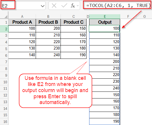
➤ Click on a blank cell where you want the consolidated column to begin (e.g., E2)
➤ Enter the following formula:
=TOCOL(A2:C6, 1, TRUE)
Here, you can replace A2:C6 with your actual range.
➤ Press Enter and the formula will spill automatically. Any blank cells present in the data will be ignored.
Consolidate Columns Using TOCOL Function (Excel 365 Only)
If you’re using Excel 365, the TOCOL function is the easiest and most efficient way to consolidate values from multiple columns into a single vertical list. It instantly stacks all the values into one column, preserving the order.
Steps:
➤ Click on a blank cell where you want the consolidated column to begin (e.g., E2)
➤ Enter the following formula:
=TOCOL(A2:C6, 1, TRUE)
Here, you can replace A2:C6 with your actual range.
➤ Press Enter and the formula will spill automatically. Any blank cells present in the data will be ignored.
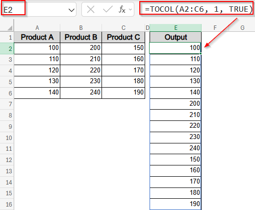
Now you have your consolidated data stacked in a single column.
Use Copy and Paste to Consolidate Columns Manually
For small datasets, the quickest way to consolidate multiple columns is by copying and pasting them one below another into a single column.
Steps:
➤ Select the first column’s data (e.g., Product A values).
➤ Press Ctrl + C to copy.
➤ Click on a blank column where you want the consolidated data (e.g., Column E, cell E2).
➤ Press Ctrl + V to paste.
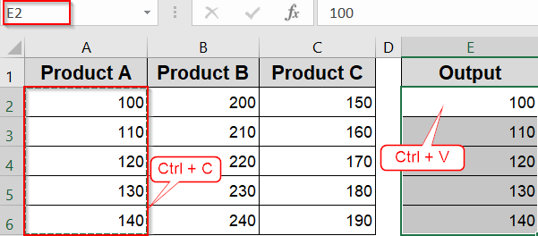
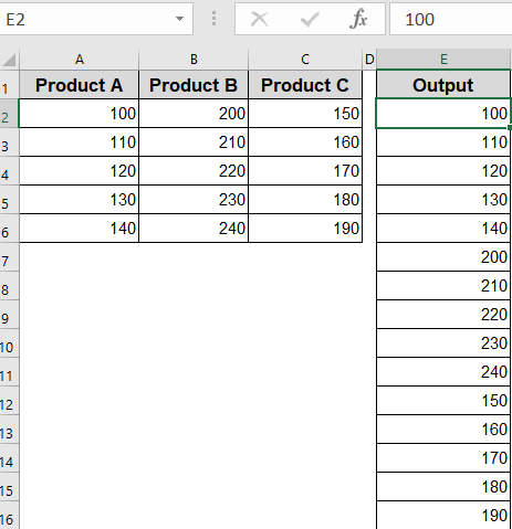
➤ Repeat for the other columns (Product B and C), but paste each below the previous data to avoid overwriting.
➤ You’ll have a single column with all values stacked vertically.
Note:
This is a static method and won’t update automatically if source data changes.
Consolidate Columns Using INDEX Function
If you want a formula that updates automatically when source data changes, the INDEX function can stack multiple columns into one. It’s ideal for dynamic, formula-based consolidation.
Steps:
➤ Choose a blank column where the consolidated list will appear.
➤ Use this formula (assuming data is in columns A to C, rows 2 to 6) in E2 cell:
=INDEX($A$2:$C$6,MOD(ROW()-ROW($E$2),ROWS($A$2:$A$6))+1,INT((ROW()-ROW($E$2))/ROWS($A$2:$A$6))+1)
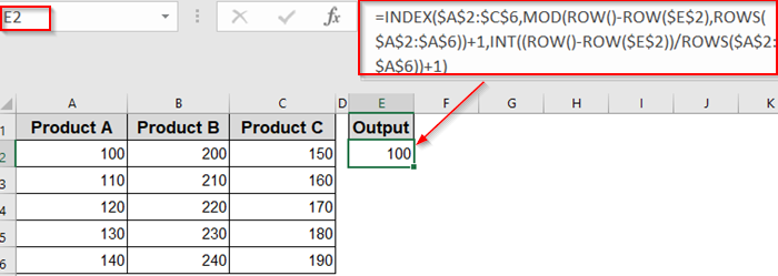
➤ Drag the formula down until all values from the three columns appear.
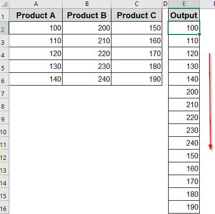
This formula cycles through each row and column to list all values sequentially.
Merge Values from Multiple Columns Using Text Formulas
If your goal is to combine values from several columns into a single cell per row, for example, merging first and last names or combining city and state text functions like CONCAT, &, and TEXTJOIN provide excellent solutions. These formulas are ideal when you want a readable, combined string from columns in the same row, and not a vertically stacked list. Let’s get started.
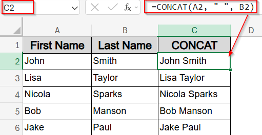
Combine Cells into One with CONCAT Function
The CONCAT function joins the contents of A2 and B2 with a space in between. This is useful when you’re combining first and last names or any values where you need custom formatting. Be aware that it does not skip blanks so you’ll need to manage spacing manually.
Steps:
➤ Select a blank cell in the same row as your data (e.g., C2).
➤ Enter the following formula:
=CONCAT(A2, ” “, B2)
➤ Press Enter.
➤ Drag the fill handle down to apply the formula to the rest of the rows.
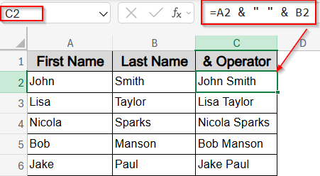
Combine Cells with the Ampersand (&) Operator
The & operator is Excel’s shorthand for joining values. This formula combines the values in A2 and B2 with a space in between. It works similarly to CONCAT but gives you more visible control, especially helpful for quick tasks or combining just two or three columns.
Steps:
➤ Click a blank cell in the same row (e.g., C2).
➤ Enter the formula:
=A2 & ” ” & B2
➤ Press Enter.
➤ Copy or drag the formula down as needed.
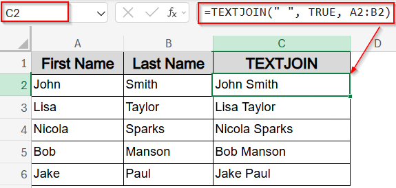
Merge Cells While Ignoring Blanks Using TEXTJOIN Function
The TEXTJOIN function joins multiple cell values using a specified delimiter, in this case, a space. The TRUE argument tells Excel to ignore any blank cells, making this ideal for names with missing middle names or optional fields. It provides the cleanest output when dealing with inconsistent or incomplete rows.
Steps:
➤ Click on a blank cell (e.g., C2).
➤ Enter this formula:
=TEXTJOIN(” “, TRUE, A2:B2)
➤ Press Enter.
➤ Drag the formula down to apply it to other rows.
Use the Built-In Consolidate Tool
Excel’s Consolidate tool lets you summarize numerical data across columns or ranges using built-in functions like SUM, AVERAGE, and more.
Steps:
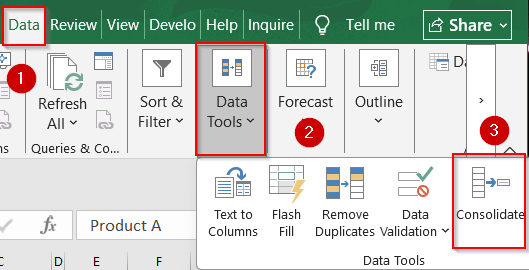
➤ Click a blank like E2 where you want your output to appear and go to the Data tab >> Click Consolidate under Data Tools.
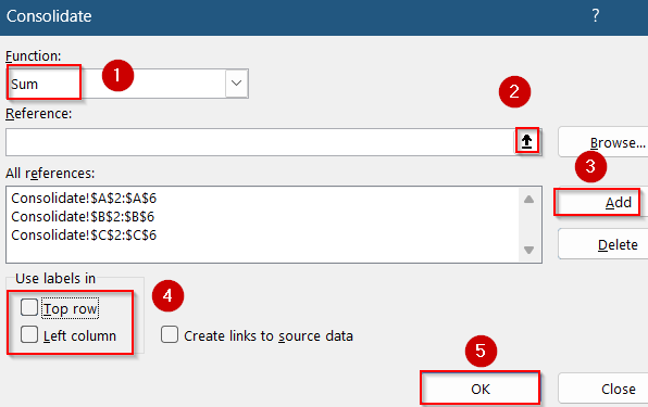
➤ Choose a function (e.g., Sum).
➤ In the Reference box, select the first data range (e.g., A2:A6) using the small arrow button and click Add.
➤ Repeat for each column (e.g., B2:B6, C2:C6).
➤ Check “Top row” and/or “Left column” if your data includes labels. Otherwise, keep it unchecked.
➤ Click OK.
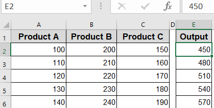
The result will show the combined values in the selected location such as E2.
Use Flash Fill to Automatically Merge Column Data
Flash Fill is perfect when you want Excel to automatically detect a pattern and combine values from multiple columns into one. It’s fast, intuitive, and great for simple merges.
Steps:
➤ In a new blank column (e.g., Column C, cell C2), manually type the desired result. For example, if A2 contains “John” and B2 contains “Smith”, type:
John Smith
➤ Press Enter.
➤ Click on cell C2 and press Ctrl + E on your keyboard, or go to the Data tab and click Flash Fill under Data Tools.
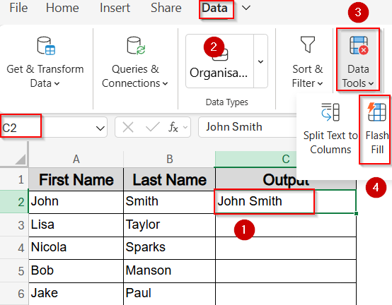
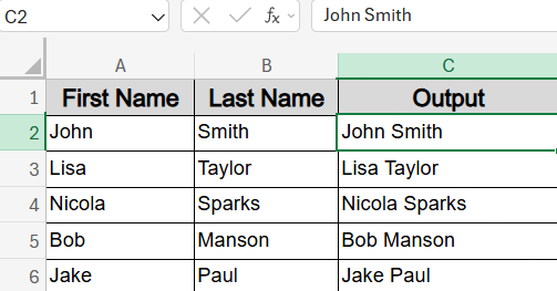
➤ Excel will instantly fill down the rest of the column by following the pattern you started.
Use Power Query to Consolidate Columns
Power Query is ideal for consolidating data from multiple columns into one column, especially with large or frequently updated datasets.
Steps:
➤ Select your data range and go to the Data tab.
➤ Click From Table/Range to load data into Power Query.
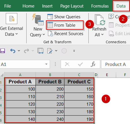
➤ Check your table has headers and click OK.

➤ In Power Query Editor, select all columns you want to consolidate.
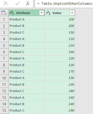
➤ Go to the Transform tab and click Unpivot Columns.
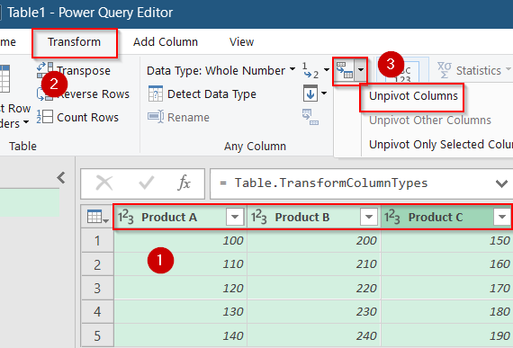
➤ This action converts multiple columns into two columns: Attribute (original column names) and Value (data).
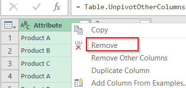
➤ Remove the Attribute column if only values are needed by right-clicking on the header.
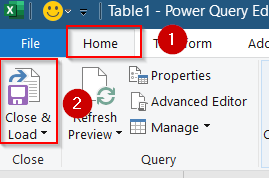
➤ Click Close & Load under Home tab to import the consolidated single column back into Excel.
Now you have a dynamic table that can refresh automatically when your source data changes.
Use VBA to Consolidate Columns Automatically
If you often need to consolidate columns from large datasets or multiple sheets, a VBA macro can automate the process quickly.
Steps:
➤ Press Alt + F11 to open the VBA editor.
➤ Insert a new module by going to Insert tab >> Module.
➤ Paste the following code:
Sub ConsolidateColumns()
Dim ws As Worksheet
Dim lastRow As Long, lastCol As Long
Dim i As Long, j As Long
Dim outputRow As Long
Set ws = ActiveSheet
lastRow = ws.Cells(ws.Rows.Count, 1).End(xlUp).Row
lastCol = ws.Cells(1, ws.Columns.Count).End(xlToLeft).Column
outputRow = 1
For j = 1 To lastCol
For i = 1 To lastRow
ws.Cells(outputRow, lastCol + 2).Value = ws.Cells(i, j).Value
outputRow = outputRow + 1
Next i
Next j
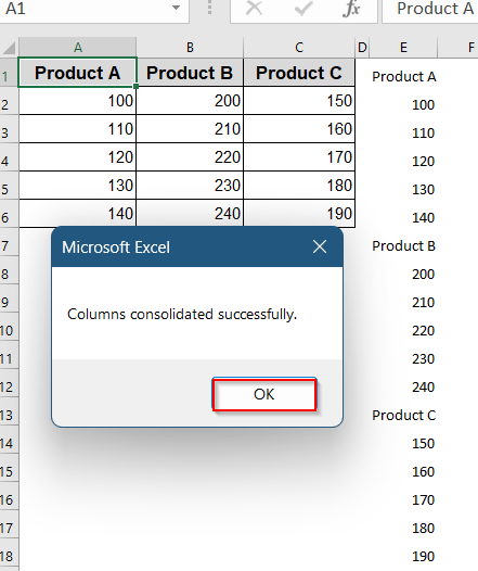
MsgBox "Columns consolidated successfully."
End Sub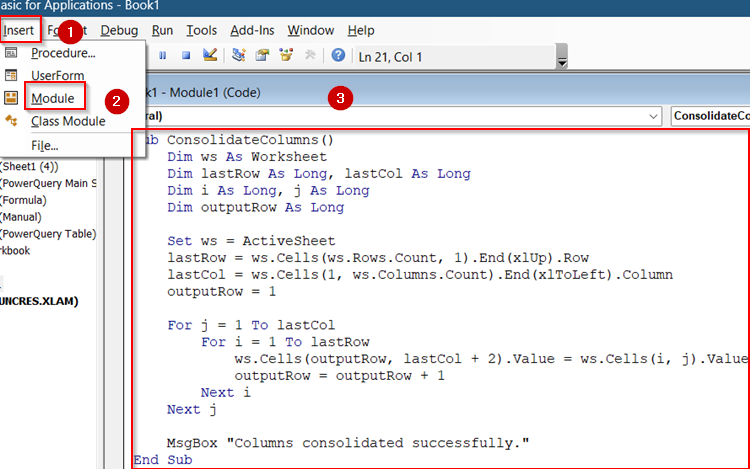
➤ Adjust the code if your data is not in the active sheet or starts at different rows/columns.
➤ Press F5 to run the macro. It will consolidate all columns into a new column located two columns right of your last data column.
➤ Click OK on the pop-up message. You’ll see that your data has appeared unformatted.
➤ Format your data accordingly by removing unnecessary header names, adjusting font, fixing alignment, etc.
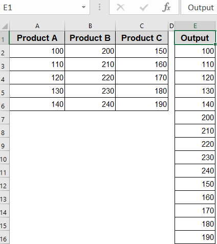
Now you have your consolidated data in a separate column arranged neatly.
Frequently Asked Questions
Which is the best formula to consolidate columns into one?
TOCOL is best if you use Excel 365. It’s clean, fast, and ignores blanks. For older versions, the INDEX + MOD + INT formula works well for dynamic stacking.
Can I consolidate data without formulas?
Yes, you can use the manual copy-paste method or the built-in Consolidate tool if you only need one-time results. These won’t update dynamically if data changes.
Can I use PivotTable to consolidate columns?
Not directly. PivotTables can summarize or group data, but don’t stack columns. You’ll need to unpivot first using Power Query, then build a PivotTable from the transformed data.
Is VBA necessary for consolidation?
Not always. VBA is useful for repetitive tasks or when dealing with large and dynamic datasets. Otherwise, built-in tools and formulas are often more than enough.
Wrapping Up
In this tutorial, we explored several effective ways to consolidate data in Excel from multiple columns ranging from manual methods to dynamic formulas like TOCOL and INDEX, as well as advanced tools like Power Query and VBA automation. Feel free to download the practice file and share your feedback.