When working with dates in Excel, you might need to add up values that fall between two specific dates. For example, you may want to calculate total sales for a product between June 1 and June 10, or only include entries from a certain region during that period.
The SUMIFS function is very useful for this. It lets you apply multiple conditions at once, such as filtering by date, product name, or region. That way, you can calculate totals that match exactly what you need.
In this article, we’ll explore several simple methods using SUMIFS along with other functions like TODAY and DATE. These methods will help you create dynamic and flexible formulas to calculate totals based on a date range and multiple criteria.
Here’s how to apply SUMIFS function to filter by date range with multiple criteria:
➤ Open your dataset in Excel
➤ Click on cell H4, where you want the result to appear.
➤ Type the following formula
=SUMIFS(E2:E11, A2:A11, “>=”&H2, A2:A11, “<=”&H3, B2:B11, H4, C2:C11, “East”)
➤ Press Enter. You’ll see the result based on the date range and the region for the product Apple.
➤ You can change East in the formula to any other region such as West, North, or South. You can also replace it with a cell reference if you want to make the region dynamic .
Use SUMIFS to Calculate Total Between Two Dates for One Product
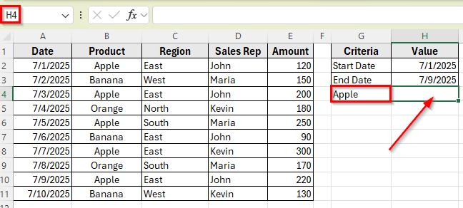
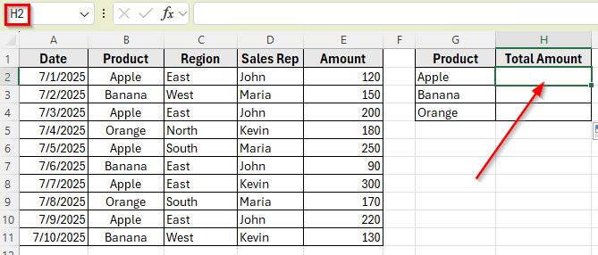
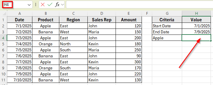
In the following dataset, we have a product sales table that includes the sale date, product name, region, sales rep, and the amount sold. The data is organized across five main columns. Column A lists the sales dates, Column B shows the product names, Column C contains the region of the sale, Column D lists the sales representatives, and Column E shows the sales amounts.
On the right side, we have a small criteria table. It includes the start date, end date, and the product we want to filter.
We’ll use this setup to calculate the total sales amount for a specific product within a given date range. The goal is to sum the values in the Amount column only if the product matches the one in cell H4 and the date falls between the start and end dates listed in cells H2 and H3.

The easiest way to calculate a total based on a date range in Excel is by using the SUMIFS function. It allows you to filter your data using two conditions for the date column. One for the Start date and one for the End date, and another condition for the Product name.
In this method, we’ll use the SUMIFS function to calculate the total sales for a specific product between two selected dates. The function will check each row to see if the date falls between June 1 and June 10, and if the product matches the one in cell G4. If both conditions are true, it will add up the values from the Amount column.
Here’s a step by step guide to apply this method:
➤ Open your dataset in Excel.
➤ Click on the cell where you want to display the total sales. For example, click on H4 next to the Product name such as Apple.
➤ Type the following formula
=SUMIFS(E2:E11, A2:A11, “>=”&H2, A2:A11, “<=”&H3, B2:B11, G4)
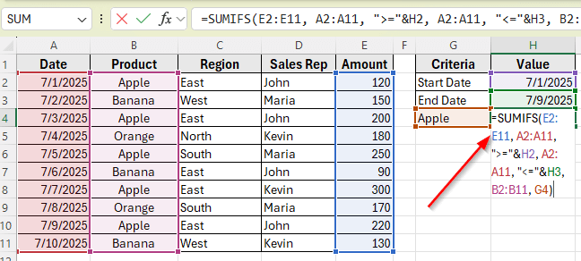
➤ Press Enter.
➤ This will return the total sales amount for Apple between June 1, 2025 and June 15, 2024. For example:
- 7/1/2025 = 120
- 7/3/2025 = 200
- 7/5/2025 = 250
- 7/7/2025 = 300
- 7/9/2025 = 220
Total= 120 + 200 + 250 + 300 + 220 = 1090
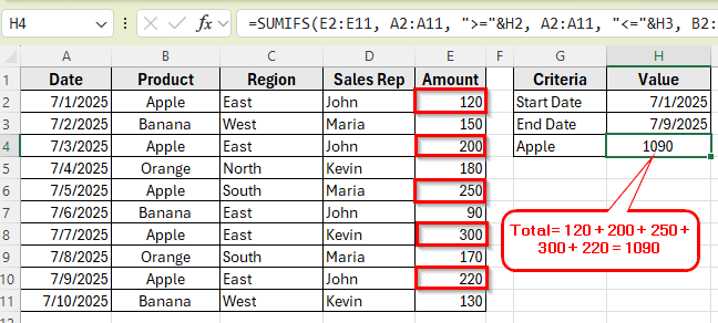
➤ You can change the product name in cell G4 to get the total for other items like Banana or Orange. The formula will update automatically.
Apply SUMIFS with TODAY Function for a Dynamic Date Range
If you want your report to always reflect the most recent data, you can use the TODAY function inside your SUMIFS formula. This method helps you create a dynamic date range that updates automatically based on the current date.
In this example, we’ll calculate total sales for a specific product in the last 7 days from today. Instead of entering the start and end dates manually, we’ll let the formula figure them out using the TODAY function.
Here’s how to apply this method:
➤ Open your Excel file.
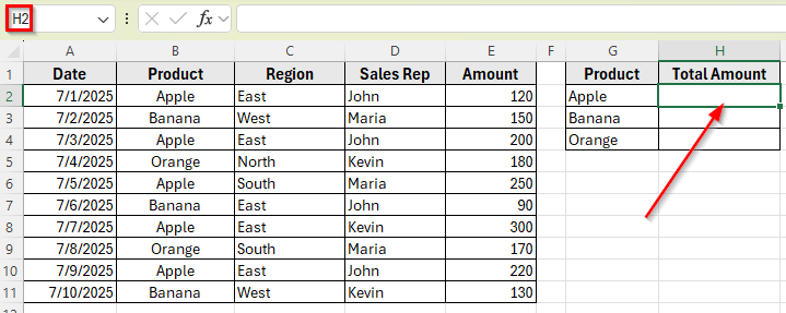
➤ Click on the cell where you want to show the total sales of Apple. For example, click on H2.
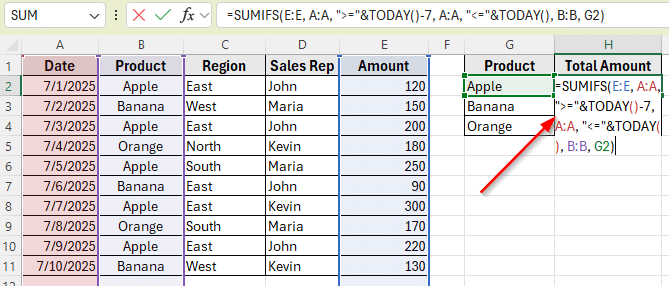
➤ Type the following formula:
=SUMIFS(E:E, A:A, “>=”&TODAY()-7, A:A, “<=”&TODAY(), B:B, G2)
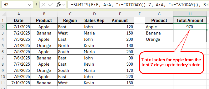
➤ Press Enter.
➤ This will display the total sales for Apple from the last 7 days up to today’s date. The formula checks if the date in Column A falls within this range and if the product in Column B matches the one in cell G2.
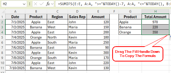
➤ Now, copy the formula for the rest of the products such as Banana and Orange, drag the fill handle down. This formula will return the total sales of both products.
Note:
Since the formula uses TODAY function, it will always reflect the latest 7-day window. So, your dataset must contain today’s actual date range.
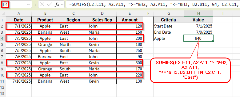
Using SUMIFS to Filter by Date Range with Multiple Criteria
Sometimes, just filtering by date is not enough. You might also want to narrow down results based on additional criteria such as a region or a sales representative. This method shows how to calculate the total sales between two dates while also including a second condition like region.
In this example, we will sum the sales for a specific product that was sold between two selected dates, and only in a specific region.
Here’s how to apply this method step by step:
➤ Open your dataset in Excel
➤ Click on cell H4, where you want the result to appear.
➤ Type the following formula
=SUMIFS(E2:E11, A2:A11, “>=”&H2, A2:A11, “<=”&H3, B2:B11, G4, C2:C11, “East”)
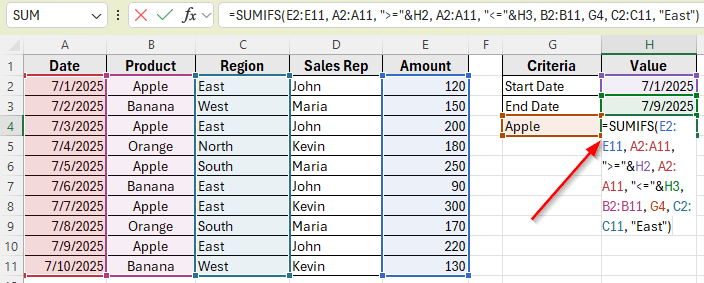
➤ Press Enter. You’ll see the result based on the date range and the region for the product Apple.
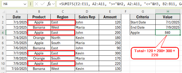
➤ You can change East in the formula to any other region such as West, North, or South. You can also replace it with a cell reference if you want to make the region dynamic
Apply SUMIFS with the DATE Function to Set Up Criteria Inside the Formula
If you do not want to use separate cells for your date inputs, you can directly write the dates inside the formula using the DATE function. This is useful when your start and end dates are fixed and not expected to change.
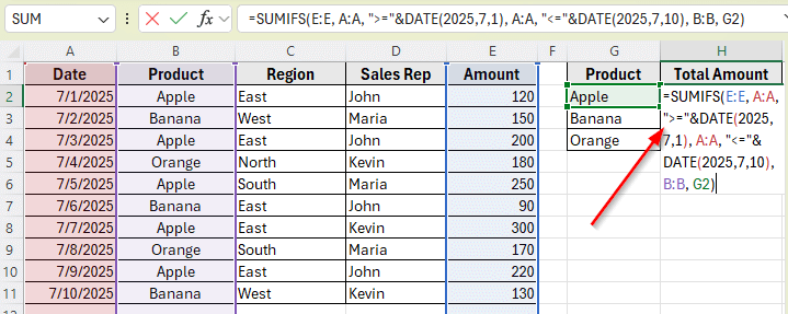
In this method, we will calculate total sales for a specific product between July 1 and July 10, 2025. Instead of referencing cells for the date range, we will use the DATE function to enter the range directly inside the formula.
Here’s how to do it:
➤ Open your dataset in Excel
➤ Click on cell H2 to calculate the total.
➤ Type the following formula
=SUMIFS(E:E, A:A, “>=”&DATE(2025,7,1), A:A, “<=”&DATE(2025,7,10), B:B, G2)
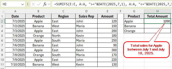
➤ Press Enter.
➤ This will return the total sales for Apple between July 1 and July 10, 2025.
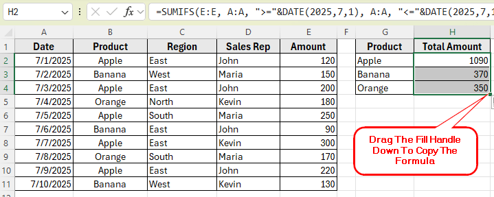
➤ Now, drag the fill handle down to copy the formula for Banana and Orange.
Frequently Asked Questions
How To Sum Values Between Two Dates In Excel?
You can use the SUMIFS function to sum values between two dates. For example, to sum sales from July 1 to July 10, use the following formula:
=SUMIFS(AmountRange, DateRange, “>=7/1/2025”, DateRange, “<=7/10/2025”)
Make sure your date values are formatted correctly so the formula returns the expected result.
How do you sum values between two dates?
To sum values between two dates in Excel, you can use the SUMIFS function. It checks if a date falls within a specific range and then adds the matching values. Here is the formula you can use it to your dataset:
=SUMIFS(E2:E11, A2:A11, “>=7/1/2025”, A2:A11, “<=7/10/2025”)
This formula adds the values from E2 to E11 only if the date in A2 to A11 is between July 1 and July 10.
Wrapping Up
The SUMIFS function gives you a lot of flexibility, especially when you need to calculate totals based on a date range in Excel. Throughout this guide, we explored different ways to make your formulas smarter. You learned how to use fixed dates, dynamic ranges with the TODAY and DATE functions. These methods allow you to create custom reports that update on their own and respond to your input changes.
You can use these formulas to build a more automated workflow. The more criteria you include, the more precise your results become.