People often use google sheets for logging activities and project management. For these jobs, it is not uncommon to have a date and time on a sheet. Sometimes, for deadlines and such, the time becomes less important than the date. For these cases, you might want to separate dates from a cell with both date and time. In this article, we will learn six ways how to remove time from date in google sheets.
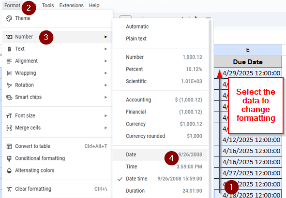
➤ Select the cells with both date and time
➤ From the menu at the top, go to Format > Number
➤ Click on “Date”
Removing time from the date isn’t always just showing the date temporarily. You might need to remove the time completely or create a new column with dates only. There are multiple methods to do all that. Stick around to learn all the methods you can use to remove time from dates in google sheets.
Changing Data Formatting
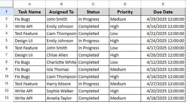
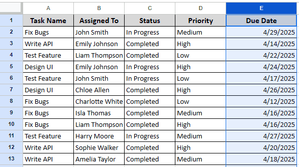
In this sample dataset, we have a bunch of deadlines for a project. You might have already noticed that all the dates have the same time. As the deadline mainly depends on the date and not the time, we don’t really need the time here. We need to remove the time to clean up the data. The following methods can be used to do just that.
The simplest method for removing time from a date in google sheets is just to change the formatting. Whenever google sheets sees that there are some dates and times in a cell, it assigns it the data type of “Date Time”. If we change it to “Date” only, the time will not be shown anymore. However, it can be restored later by changing the formatting back to the original.
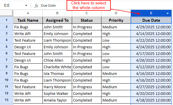
➤ Select all the cells that you need to modify. You can use your mouse to drag and select the cells, or you can click the column name to select the whole column.
➤ Go to the “Format” menu, and head to Number > Date.
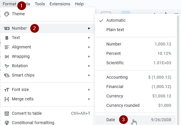
➤ Now the selected column will only show the date instead of the date and time.
Extracting Only Date from Date and Time
In this method, we will extract the date from the column with the date and time to another column. This can be helpful if you want to have the date and time in one column, and only the date in another. Follow the steps below:
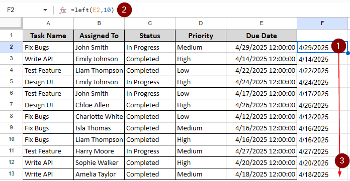
➤ Select another column to extract the date. In this example, we are choosing the column right next to the column with the date and time. The date and time start with the E2 cell, and we are writing the date from the F2 cell.
➤ Write this formula there:
=LEFT(E2,10)
➤ Now, drag the cell to the bottom to autofill the formula to all cells.
Splitting the Text
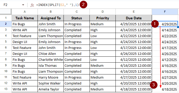
In the table, there is a space between the date and the time. We will use the space as a marker to split the date and time and extract the date only.
➤ We will need a helper column here as well, and we are choosing the F column like the previous example.
➤ Go to the F2 cell, and write this formula:
=INDEX(SPLIT(E2," "),1)
➤ You might need to set the formatting to Date like method 1 if you see numbers only.
➤ Autofill the formula in the other cells as you did before.
Rounding Up the Number
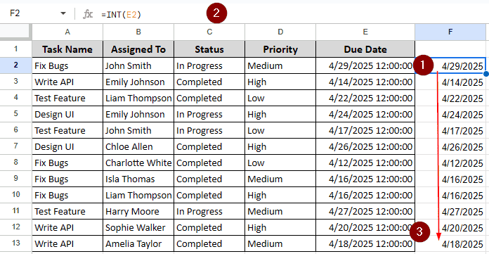
Using another formula, we can round the number from the date and time. Google Sheets stores the time as a fractional number. If we get rid of that, we are left with the date only.
➤ Take a helper column. Set the data formatting to date.
➤ Write the formula to the first cell (other than the heading).
=INT(E2)
➤ Autofill the formula to other cells.
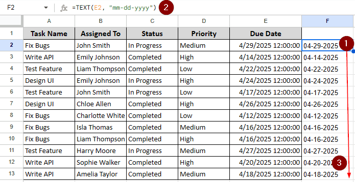
Extracting Text with Format
In this method, not only can we extract the date, but change the formatting of the date as well. Just follow the steps given below:
➤ Go to another column with the same rows (that will help with auto-filling)
➤ Write the formula:
=TEXT(E2, "mm-dd-yyyy")
➤ Autofill the other cells. You don’t need to change the cell format as the function outputs plain text.
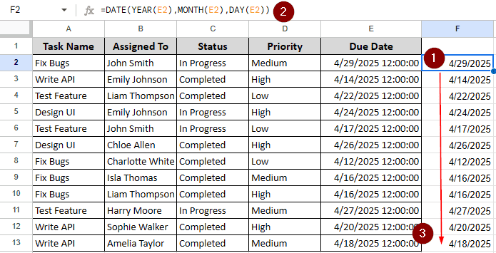
Using the Date Function
Using the DATE function to extract the date should be an obvious choice. We will need a helper column with it in order to extract the data to that column.
➤ You know the drill by now, take another column near the date with the same row, and enter this formula:
=DATE(YEAR(E2),MONTH(E2),DAY(E2))
➤ Autofill the other cells. You do not need to change the formatting of the cells as the DATE function automatically does that for you.
Frequently Asked Questions
How do I remove time from date format in excel?
Select the cell you want to work with. Then right click, and select “Format Cells”. From the “Number” tab, select Date. Choose your preferred date format without time, and click OK.
How do I change the date format in Sheets?
From the “File” menu, go to “Spreadsheet settings”. Then change the locale to your native (or the one you want) and save.
How do I deduct time in Google Sheets?
Use the minus (-) sign to subtract the time, as the time is stored in fraction format. The formula should be like this:
=A2-B2
Then change the cell formatting to time.
How do I fix time in Google Sheets?
If the time does not show up properly, it is probably a sign of having a time zone difference. Go to “Settings” from the “File” menu. Then go to General > Locale > Time zone and choose your preferred time zone.
How to separate time from date in Google Sheets?
We can use subtraction and rounding up to do that. Use this formula:
=A1-INT(A1)
Here, the INT function rounds up the number, which is the date, and subtracts it from the date and time. Then change the cell formatting to time, and you are done.
Wrapping Up
In this article, we have learned six methods on how to remove time from a date in google sheets. Hope you learned something from the article. Use the practice file to understand the methods better, and leave a comment on how you found this helpful to your job.