How to Create a Dependent Drop-Down List in Google Sheets

When working with dropdowns in Google Sheets, sometimes having just one list of values is not enough. You may want a second dropdown to dynamically update its options based on what’s selected in the first one. This type of setup is known as a dependent drop-down list.

Let’s say you’re managing employee data. After choosing a department, you want the next column to show only the roles in that department. A dependent drop-down does that, making your data entry process smoother, faster, and more accurate.

What Is a Dependent Drop-Down List in Google Sheet?

A dependent drop-down list allows you to change the options in one cell based on the selection made in another. This requires a workaround using named ranges and the INDIRECT function in Google Sheets.

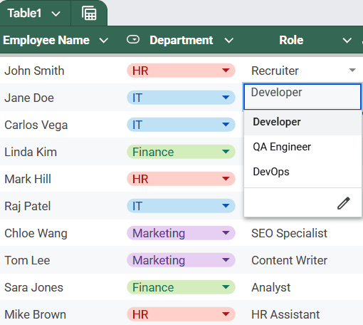
For example, if “IT” is selected as a department, the roles column only shows options like Developer, QA Engineer, or DevOps, hiding irrelevant choices.

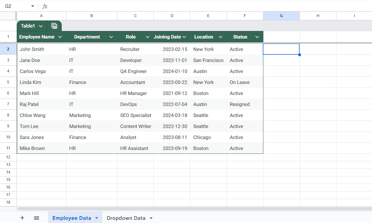
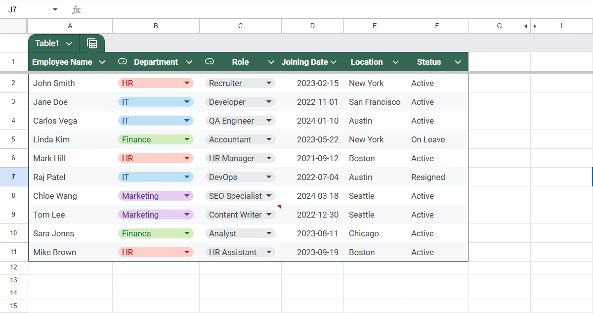
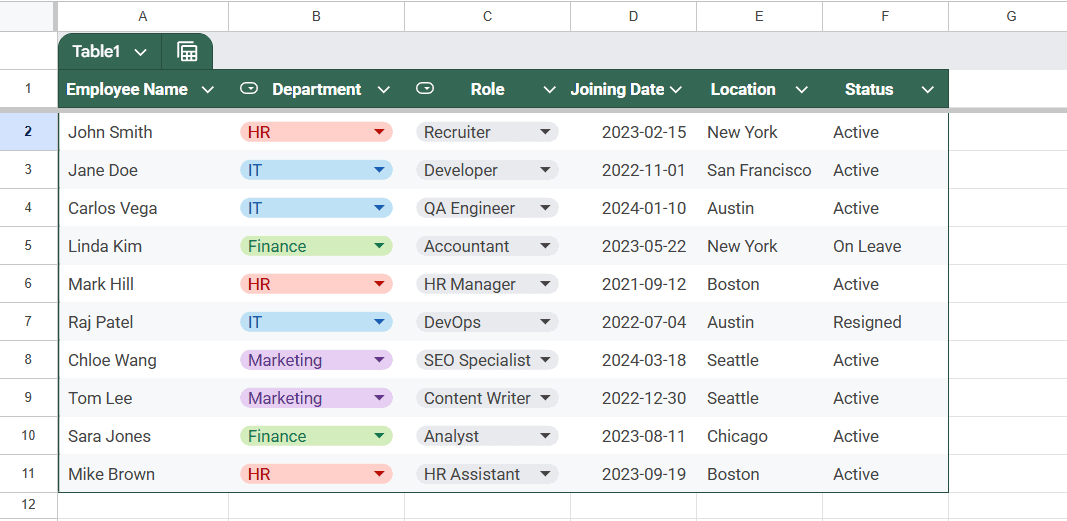
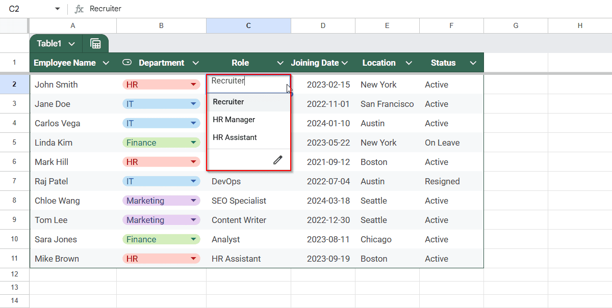
In the following dataset, we are managing employee information across different departments. After selecting a department from a drop-down, we want the “Role” column to update based on the selected department.

Prepare the Reference Table

Steps:

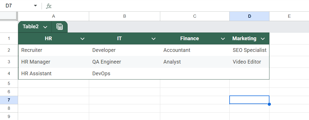
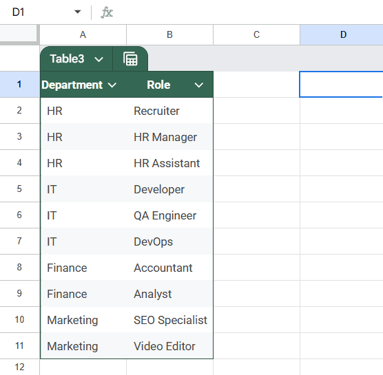
➤ Create a reference sheet named Dropdown Data that lists departments and the roles under each.

Name the Role Ranges

To make the dependent dropdowns work, you need to name each row of roles.

Steps:

➤ Select the cells B2:D2 (roles for HR)
➤ Go to Data >> Named ranges

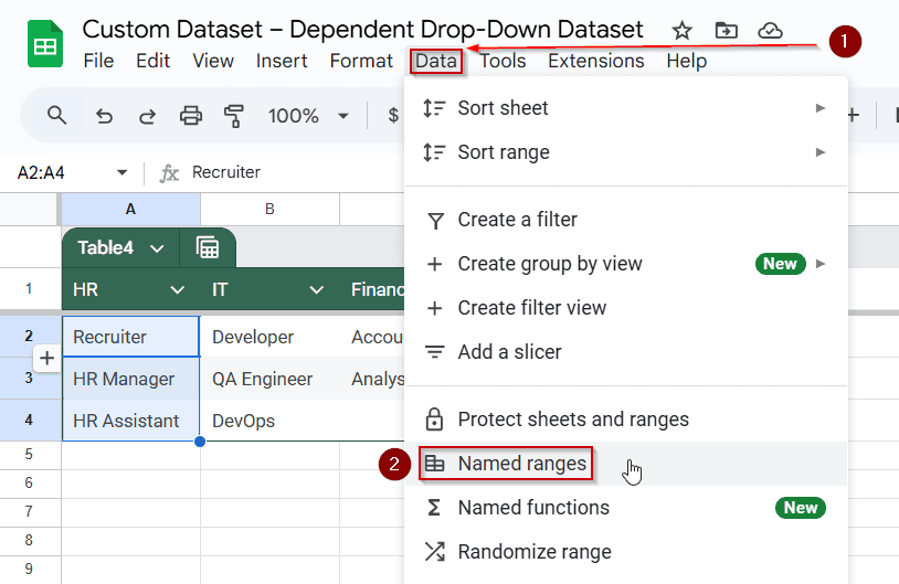
➤ Name the range as HR

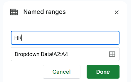
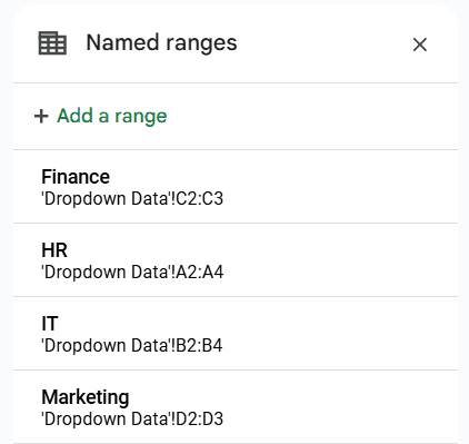
➤ Repeat the process for other rows (e.g., IT, Finance, Marketing)

Set Up the Main Table

Now go to the sheet where you want the dropdowns to appear, let’s say it’s named Employee Data.

Create the First Drop-Down (Department)

Steps:

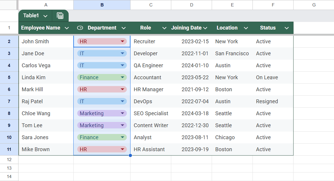
➤ Select the cells under the “Department” column
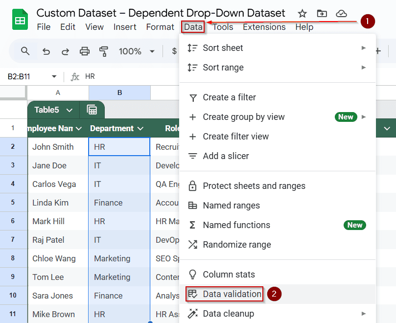
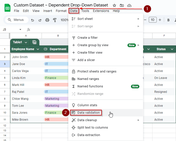
➤ Go to Data >> Data validation

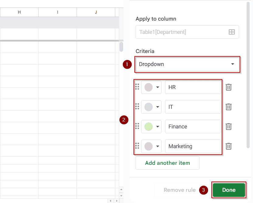
➤ Choose the Dropdown from the criteria
➤ Enter these values manually: HR, IT, Finance, Marketing

➤ Click Done

Create the Dependent Drop-Down (Role)

Steps:

➤ Set a helper column (e.g., column H)
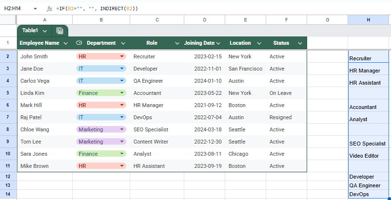
➤ In H2, use:

➤ Drag this down formula down to H14

Then, apply data validation in C2:C11 to refer to range H2:H14

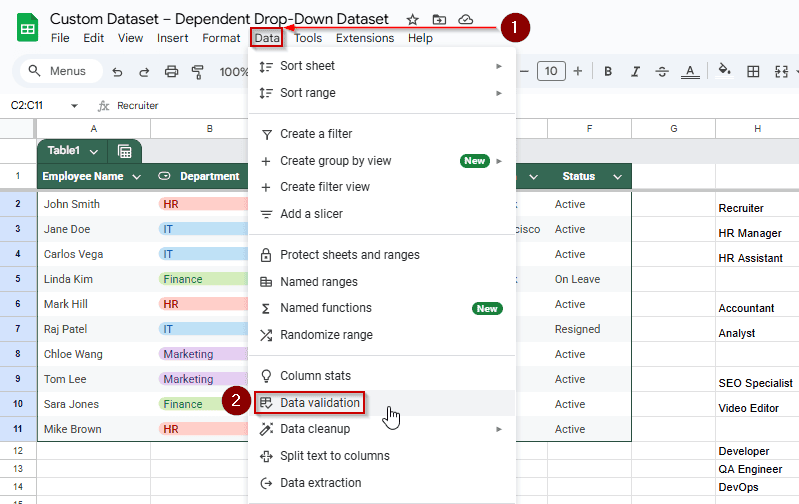
➤ Select the cells under the “Role” column
➤ Go to Data >> Data validation

➤ Choose Dropdown
➤ Set the criteria to “Dropdown from range”
➤ Input the range into the box: H2:H14
➤ Apply the rule to the entire column if needed
➤ Click Done
➤ Hide the helper column.

If your category names include spaces, or if you want a solution that doesn’t rely on named ranges, use this method.

Structure Your Reference Table Vertically

Instead of placing roles side-by-side, list them vertically:

Create Department Drop-Down (Same as Before)

➤ Use manual entry for departments in Column B of your main sheet:

Use FILTER Function in a Helper Column

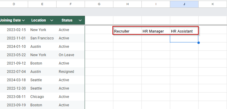
➤ In a hidden or side column (say column H), use the following formula In H2:

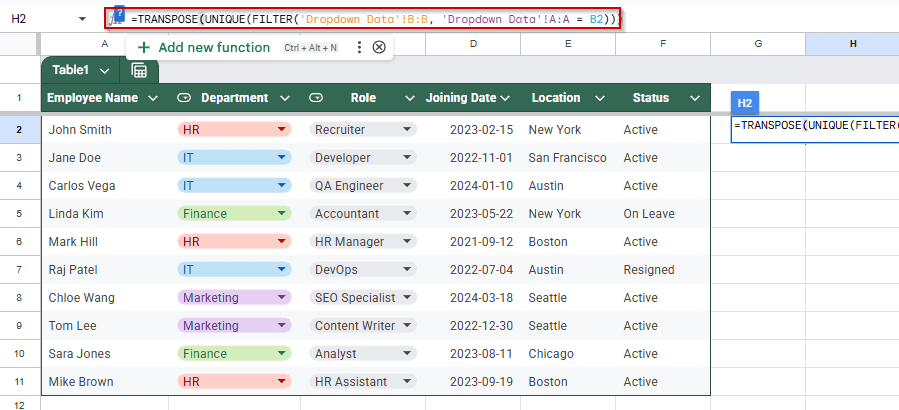
This pulls roles for the department selected in B2 and transposes them horizontally.

➤ Pull the formula down from cell H2 until H11.
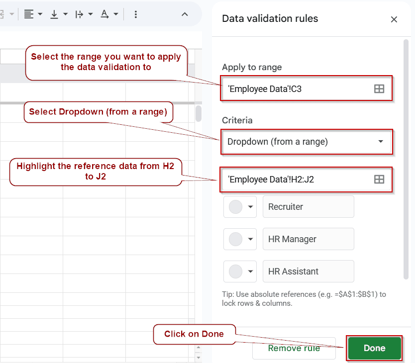
➤ Go to Data >> Data validation

➤ Select “Dropdown (from a range)”

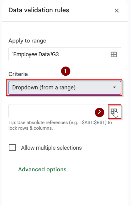
➤ Click on the small table icon, the Select data range button
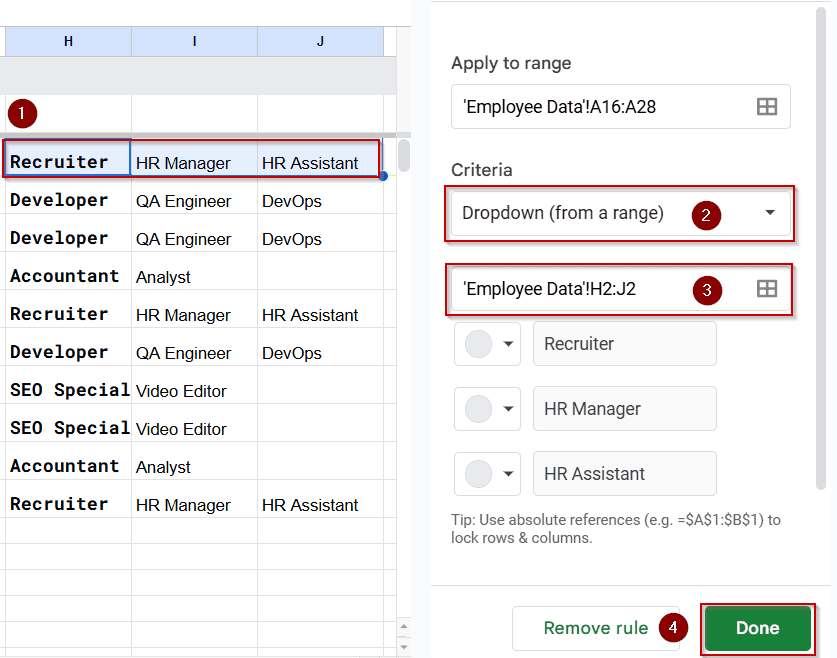
➤ Select the cells from H2
➤ The different roles should be selected on the right.
➤ Verify if it’s correct, and click on Done.

➤ Do the same for all departments.

This is the most efficient way of doing dependent drop-downs. We will be using the same sheets that we used previously.

Open Apps Script

➤ In Google Sheets, go to Extensions >> Apps Script

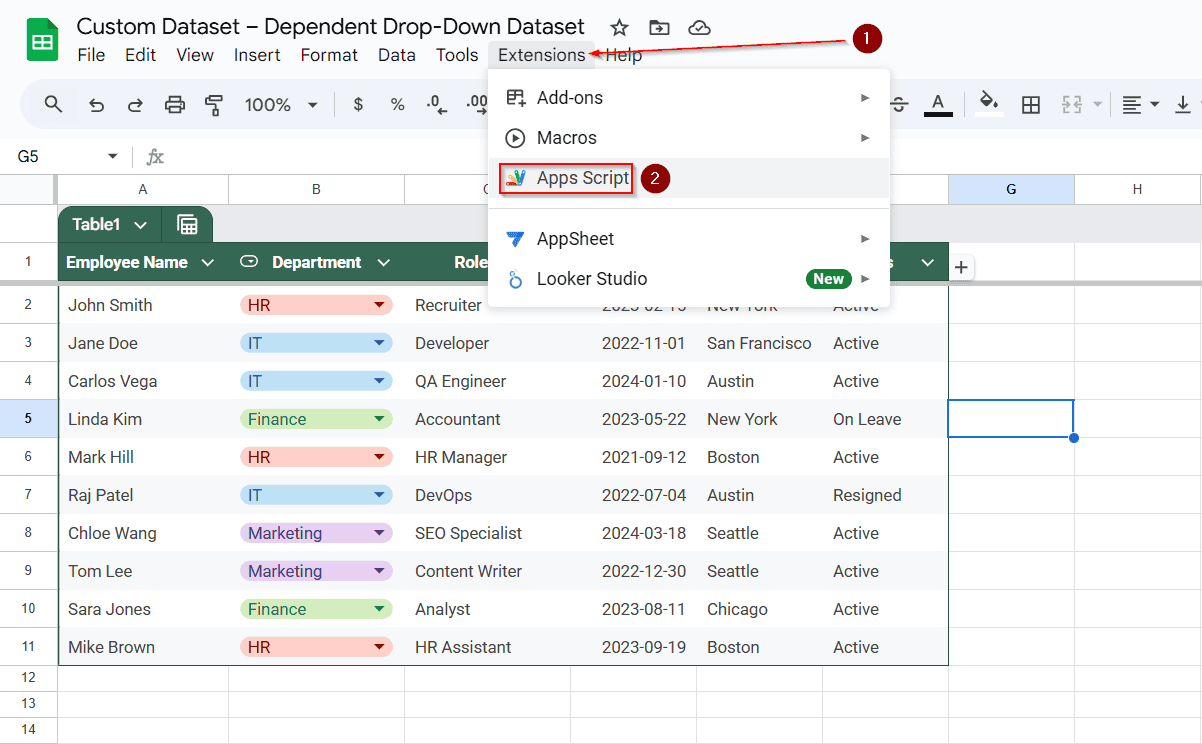
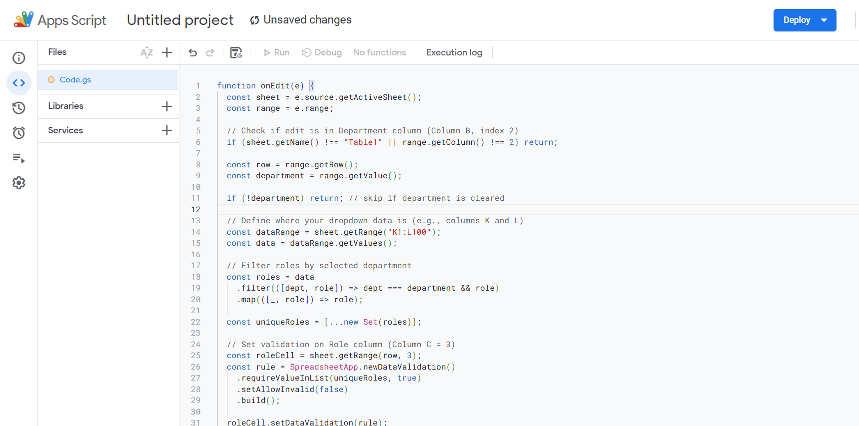
➤ Delete any existing code and paste the code below:

function onEdit(e) {
if (!e) return;
const sheet = e.range.getSheet();
if (sheet.getName() !== "EmployeeData") return;
const editedCell = e.range;
const editedColumn = editedCell.getColumn();
const editedRow = editedCell.getRow();
// Proceed only if the edited cell is in column B (Department) and not the header row
if (editedColumn === 2 && editedRow > 1) {
const department = editedCell.getValue();
// Retrieve the mapping table from columns K and L
const dataRange = sheet.getRange("K1:L100").getValues();
// Filter roles corresponding to the selected department
const roles = dataRange
.filter(row => row[0] === department)
.map(row => row[1])
.filter(role => role); // Remove any empty values
// Create a data validation rule with the filtered roles
const rule = SpreadsheetApp.newDataValidation()
.requireValueInList(roles, true)
.setAllowInvalid(false)
.build();
// Apply the data validation to the corresponding cell in column C (Role)
sheet.getRange(editedRow, 3).setDataValidation(rule);
}
}

Save and Authorize

Steps:

➤ Click on File >> Save (name it something like DependentDropdown)
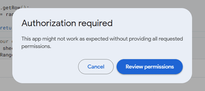
➤ Click Run >> onEdit once (it will ask for permissions)

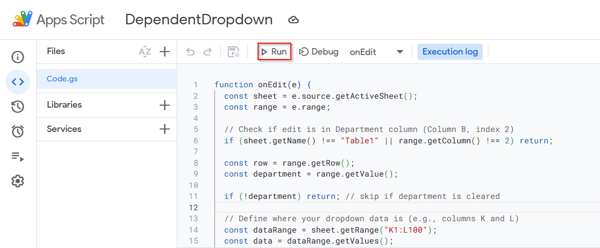
➤ Grant permission using your Google account

Test It Out

Back in your sheet:

➤ In column B, select a department (e.g., “HR”).
➤ Column C will instantly become a dropdown showing roles related to “HR” only.

Clear Old Role if Department Changes

To prevent mismatched roles when departments change, replace the line:

const roleCell = sheet.getRange(row, 3);

with:

const roleCell = sheet.getRange(row, 3);
roleCell.clearContent(); // Clear old role

Frequently Asked Questions

How do I update or expand a role list later?

You can expand the named range for any department from Data >> Named ranges. Simply adjust the range to include new cells, and the dependent dropdown will update automatically.

Can I apply this across multiple rows?

Yes, once the formula is set for one row, you can apply it to others. Just ensure the formula always refers to the cell in the same row (e.g., =INDIRECT(B3) for Row 3.)

What happens if I delete a named range?

The dependent drop-down will stop working and may return an error. Be sure not to delete named ranges unless you’re updating them.

Is there a way to do this without named ranges?

There are alternatives using Google Apps Script or helper tables with FILTER() functions, but named ranges with INDIRECT() are the most accessible method for most users.

Wrapping Up

Creating dependent drop-down lists in Google Sheets can drastically improve data accuracy and streamline your workflow, especially when managing structured data like employee records. Whether you prefer using simple named ranges with the INDIRECT function, dynamic formulas like FILTER, or more advanced automation with Google Apps Script, there’s a method to suit every level of expertise. Choose the approach that fits your data best and you’ll have smarter, cleaner spreadsheets in no time.