If you’re managing lists, forms, or trackers in Google Sheets, it’s often useful to automatically fill in a value in one column based on the input in another. For example, selecting a product code could auto-fill the product name or price in another cell.
In this article, you’ll learn how to use built-in functions like VLOOKUP, IF, ARRAYFORMULA, and Google Apps Script to set up smart autofill workflows in your sheet.
Steps to autofill based on another field in Google Sheets:
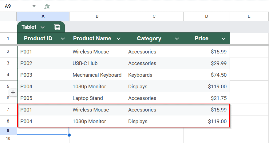
➤ In your sheet, set up a reference table in cells A1 to D6 with columns for Product ID, Product Name, Category, and Price.
➤ Below the reference table (starting at A8), type or paste the new Product IDs you want to look up.
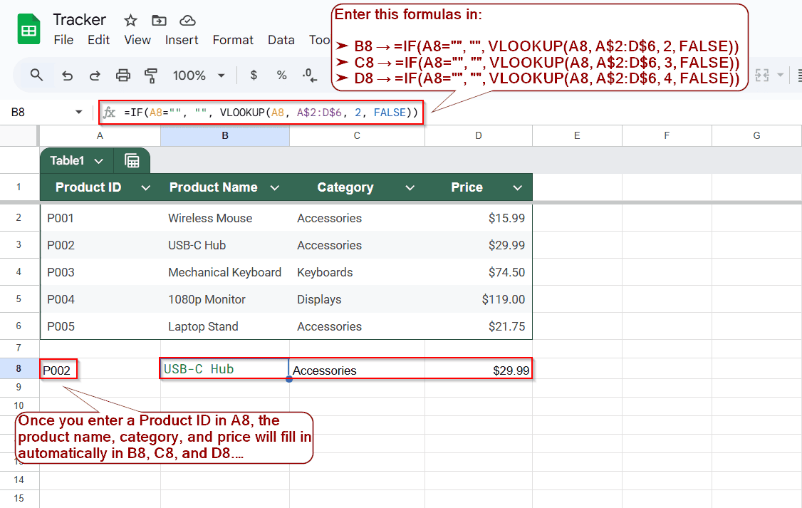
➤ In cell B8, enter this formula to fetch the Product Name: =IF(A8=””, “”, VLOOKUP(A8, A$2:D$6, 2, FALSE))
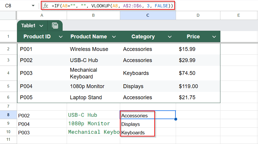
➤ In C8, get the Category using: =IF(A8=””, “”, VLOOKUP(A8, A$2:D$6, 3, FALSE))
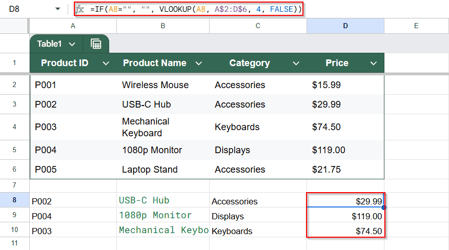
➤ In D8, autofill the Price: =IF(A8=””, “”, VLOOKUP(A8, A$2:D$6, 4, FALSE))
➤ Drag all three formulas to apply them across as many rows as needed.
Use the VLOOKUP Function to Autofill Based on a Product ID
The VLOOKUP function is one of the simplest and most effective tools for autofilling data in Google Sheets based on a single input field, in this case, a Product ID. It works by searching for the input value in the first column of a reference table and returning related data from a column to the right.
This method is perfect when you have a structured product list or any kind of lookup table, and you want other columns to populate automatically when someone selects or types a code.
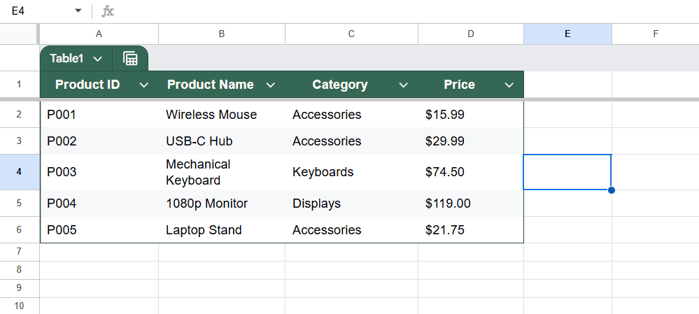
We’ll use the following dataset on a sheet called Product Tracker to demonstrate to you how this method works:
This highly scalable approach doesn’t require scripting, making it ideal for beginners or anyone building an inventory, order form, or product selector.
Steps:
➤ Set up your reference table in cells A1 to D6 as shown in the screenshot above
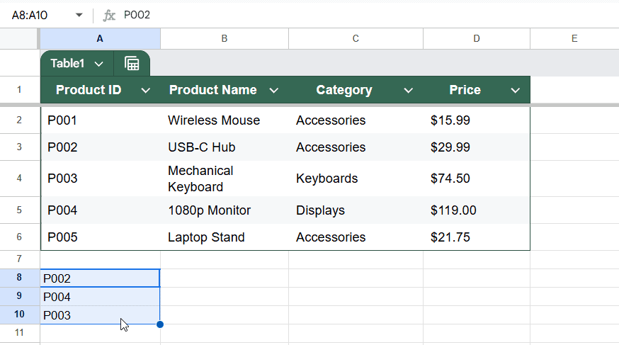
➤ Below the table, starting in row 8, enter Product IDs in Column A.
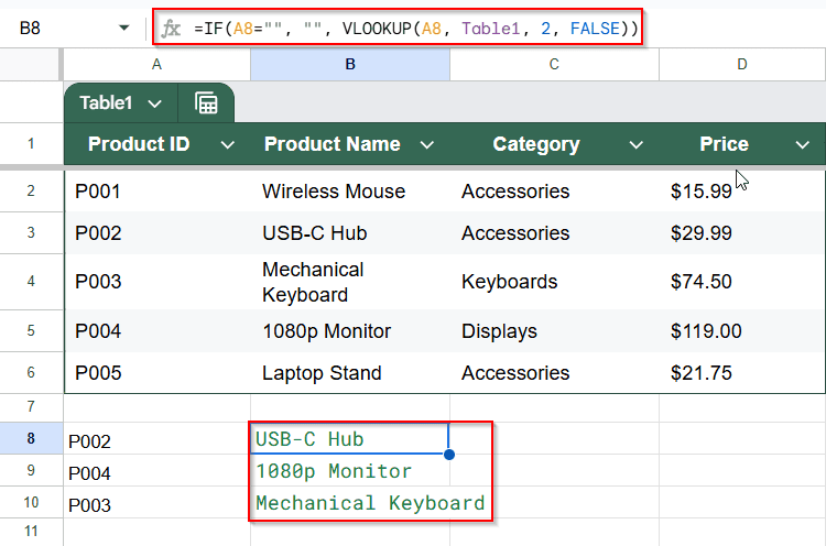
➤ In B8, enter this formula to fetch the product name:
=IF(A8=””, “”, VLOOKUP(A8, A$2:D$6, 2, FALSE))
➤ In C8 (Category), use:
=IF(A8=””, “”, VLOOKUP(A8, A$2:D$6, 3, FALSE))
➤ In D8 (Price), use:
=IF(A8=””, “”, VLOOKUP(A8, A$2:D$6, 4, FALSE))
➤ Drag these formulas down to apply them to more rows.
This method works best when your reference table is static and your lookup values are unique, like IDs or SKUs.
Autofill Across Rows Using ARRAYFORMULA Function
The ARRAYFORMULA function lets you apply a formula to an entire column at once. It removes the need to drag formulas down manually and updates automatically as users enter new values.
We’ll use the same Product Tracker sheet. When a Product ID is typed into Column A, the product name, category, and price will automatically appear in Columns B, C, and D using ARRAYFORMULA. This is useful for forms, templates, or any growing list of entries.
Steps:
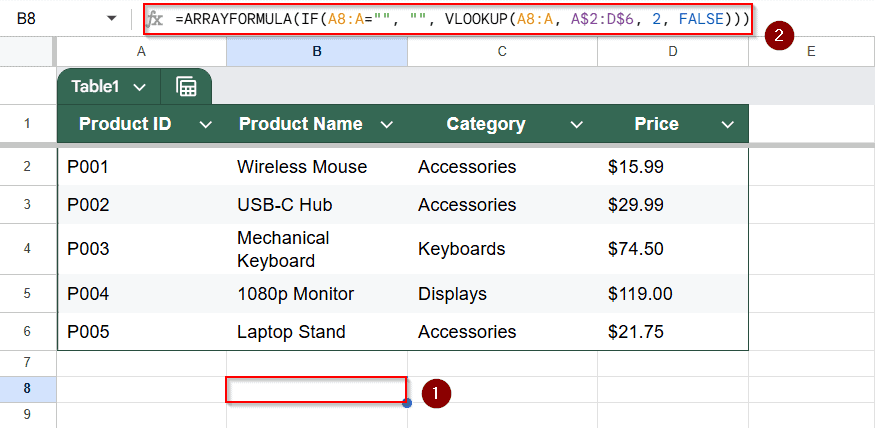
➤ In Column B (Product Name), enter this formula in B8:
=ARRAYFORMULA(IF(A8:A=””, “”, VLOOKUP(A8:A, A$2:D$6, 2, FALSE)))
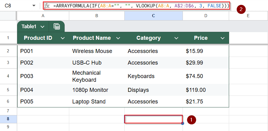
➤ In cell C8 (Category), enter:
=ARRAYFORMULA(IF(A8:A=””, “”, VLOOKUP(A8:A, A$2:D$6, 3, FALSE)))
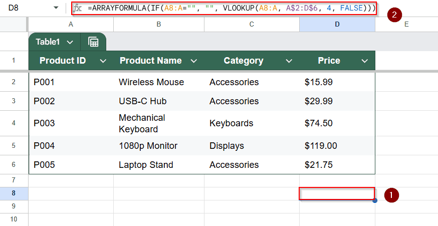
➤ In cell D8 (Price), enter:
=ARRAYFORMULA(IF(A8:A=””, “”, VLOOKUP(A8:A, A$2:D$6, 4, FALSE)))
➤ Now you can enter Product IDs starting from cell A2 downward, and Columns B, C, and D will fill automatically as long as the matching ID exists in your reference table.
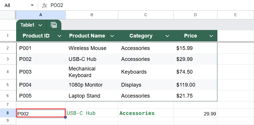
This is a hands-free method for auto-populating data in real time as entries are added. Let me know if you’d like a version that excludes blank rows or stops at a specific limit.
Apply Conditional Autofill Using IF Statements
The IF function is proper when you only have a few known inputs and want to return custom outputs based on those. It’s a simple way to autofill values like product names or categories without creating a complete lookup table.
This method works well when the data options are limited and clearly defined.
We’ll use a simplified version of your product list. In Column A, the user will enter a Product ID, and in Column B, the corresponding Product Name will automatically appear using an IF formula.
Steps:
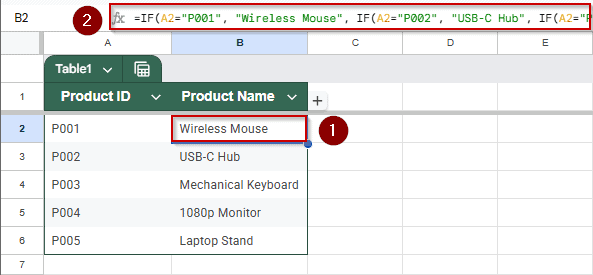
➤ In cell B2, enter this formula:
=IF(A2=”P001″, “Wireless Mouse”, IF(A2=”P002″, “USB-C Hub”, IF(A2=”P003″, “Mechanical Keyboard”, IF(A2=”P004″, “1080p Monitor”, IF(A2=”P005″, “Laptop Stand”, “”)))))
➤ Drag the formula down to apply it to more rows.
This method is best used when you only have a few IDs to manage and want a quick solution without needing a reference table or advanced functions.
Create Custom Autofill Rules Using Apps Script
When formulas aren’t flexible enough, Google Apps Script gives you full control to create advanced autofill behavior. You can write a script that reacts whenever a specific cell is edited and then fills in related information automatically.
This method is ideal when you want to remove formulas from the sheet, apply custom rules, or update multiple columns based on a single input. It runs in the background and updates values instantly, without requiring user action beyond typing a value.
Steps:
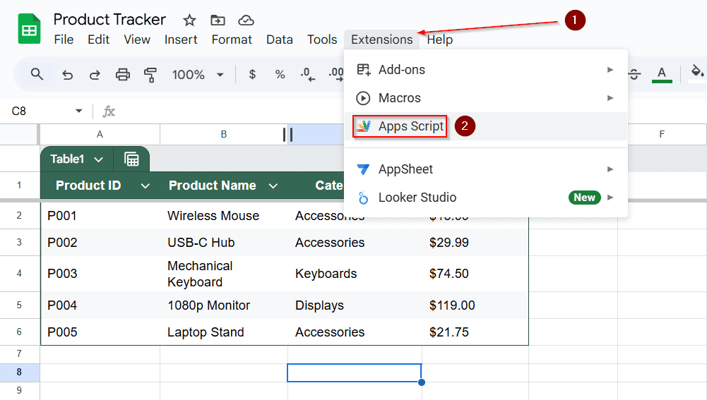
➤ Go to Extensions >> Apps Script
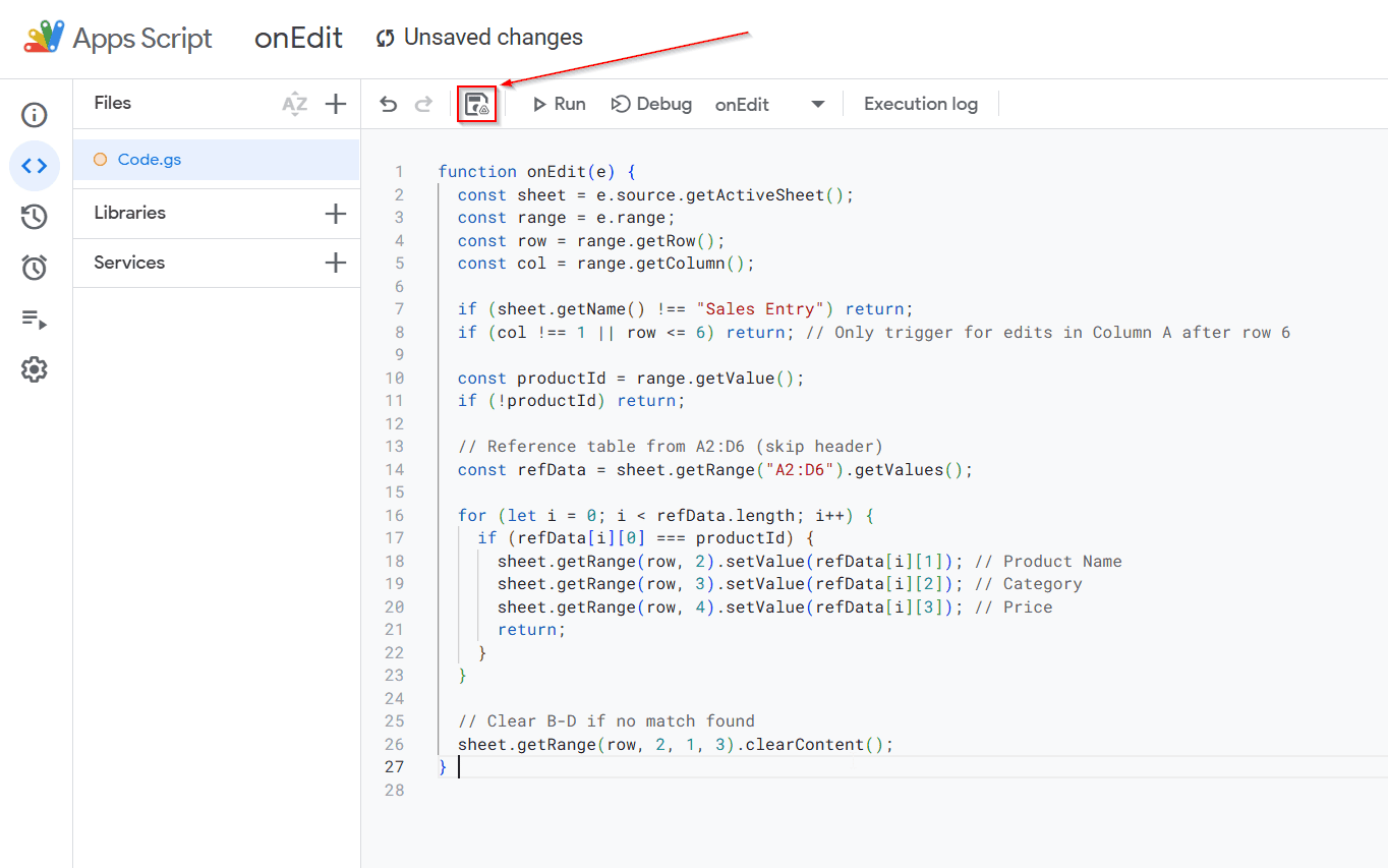
➤ Paste this script:
function onEdit(e) {
const sheet = e.source.getActiveSheet();
const range = e.range;
const row = range.getRow();
const col = range.getColumn();
if (sheet.getName() !== "Sales Entry") return;
if (col !== 1 || row <= 6) return; // Only respond to Column A after row 6
const productId = range.getValue();
if (!productId) return;
// Your reference data is in A2:D6
const refData = sheet.getRange("A2:D6").getValues();
for (let i = 0; i < refData.length; i++) {
if (refData[i][0] === productId) {
sheet.getRange(row, 2).setValue(refData[i][1]); // Product Name
sheet.getRange(row, 3).setValue(refData[i][2]); // Category
sheet.getRange(row, 4).setValue(refData[i][3]); // Price
return;
}
}
// If no match, clear any existing values
sheet.getRange(row, 2, 1, 3).clearContent();
}
➤ Save the script by clicking on the floppy disk icon and return to the sheet.
➤ When you type a Product ID in Column A, the rest will autofill automatically.
This is best when you want to remove formulas and fully automate the logic behind the scenes.
Frequently Asked Questions
How can I autofill data in Google Sheets without dragging?
Use ARRAYFORMULA to apply a formula across a range. For example: =ARRAYFORMULA(IF(A2:A=””, “”, A2:A * 2)) applies the formula to all rows without manual dragging.
How do I autofill based on another sheet’s data?
Utilize VLOOKUP to reference another sheet. Example: =VLOOKUP(A2, ‘Sheet2’!A:B, 2, FALSE) fetches corresponding data from ‘Sheet2‘ based on the value in A2.
Can I autofill using conditional logic?
Yes, employ IF or IFS functions. For instance: =IF(A2=”US”, “United States”, IF(A2=”EU”, “Europe”, “”)) returns specific values based on the condition in A2.
How does Smart Fill work in Google Sheets?
Smart Fill detects patterns and suggests autofill options. Start typing in a cell; if a pattern is recognized, press Ctrl + Shift + Y to accept the suggestion.
How can I autofill dates or sequences automatically?
Enter the initial values to establish a pattern, then use the fill handle to drag and autofill. Google Sheets continues the sequence based on the identified pattern.
Wrapping Up
Google Sheets offers flexible ways to autofill data based on another field, from simple VLOOKUP formulas to fully scripted automation. Whether you’re building a form, tracking sales, or creating a product entry log, the correct method depends on how dynamic and scalable your sheet needs to be.
Use formulas for fast setups, and consider Apps Script if you’re building something more advanced or automated.