If you’re working with financials, reports, or regional data in Google Sheets, using custom number formats can dramatically improve how your spreadsheet looks, without changing the underlying values. Instead of seeing plain numbers, you can show dollars, percentages, shortened thousands (K), or even attach units like “days” or “kg.”
In this article, you’ll learn how to apply custom formats using Google Sheets’ built-in options. We’ll also walk through real examples using a sample dataset.
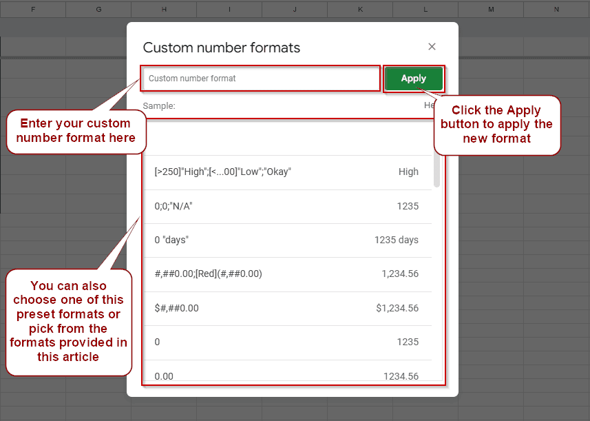
Steps to apply custom number formats in Google Sheets:
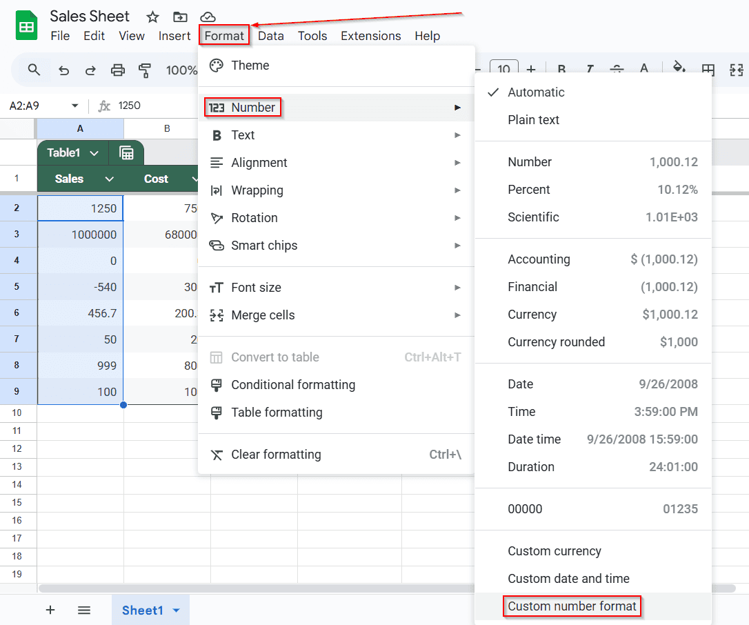
➤ Use Format >> Number >> Custom number format
➤ Enter a format using codes like 0, #, “text”, and @
➤ Define different display styles for positive, negative, zero, and text
➤ You can apply colors with brackets like [Red]
➤ Custom formats control how values look, but not the values themselves
Show Leading Zeros for Codes or IDs on Google Sheet
When working with ID numbers, zip codes, or product codes, you should make all the numbers look consistent, even if they have different lengths. Google Sheets removes leading zeros by default (so 00123 turns into 123), but with a custom number format, you can force those zeros to appear for display purposes.
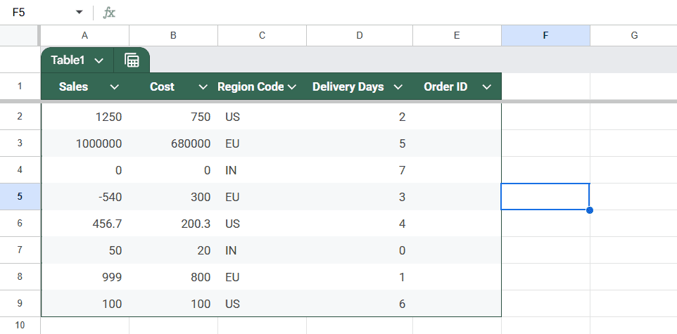
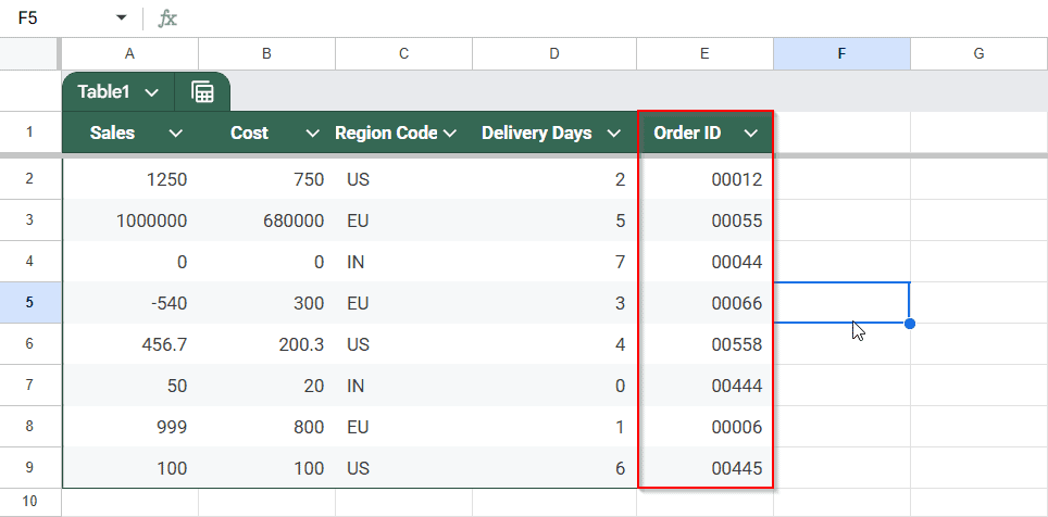
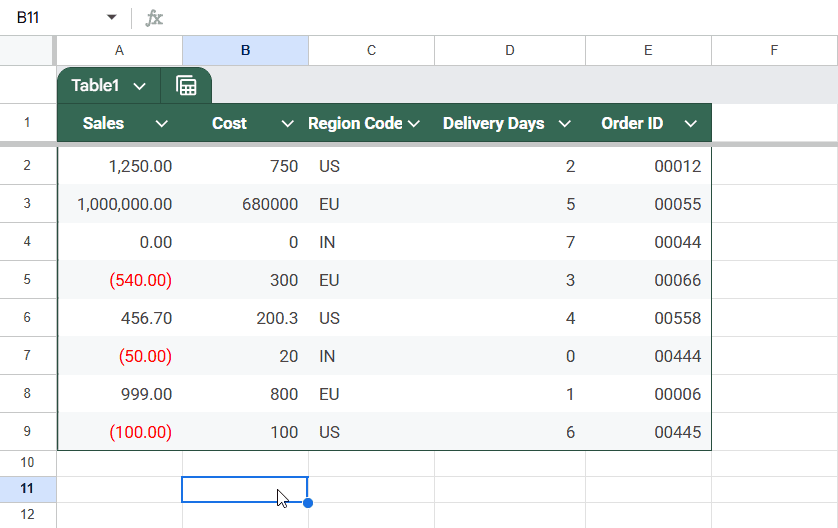
We’ll use a Sales Report sheet for this example. Let’s say you’ve added a new column named Order ID in Column E with values like 1, 23, or 456. To make every ID display a 5-digit code (e.g., 00001, 00023, 00456), follow the steps below.
Steps:
➤ Select the cells in Column E (Order ID)
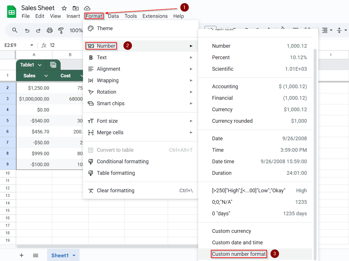
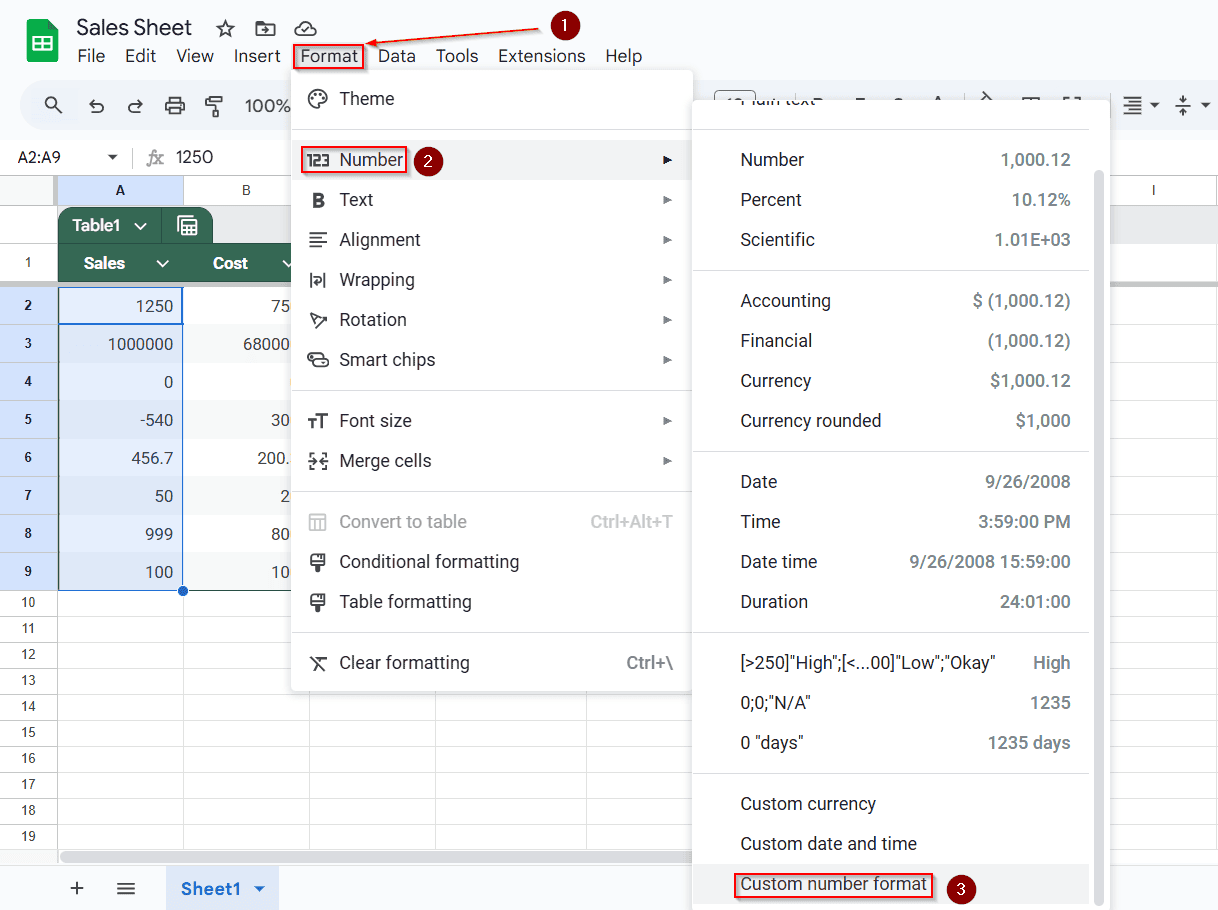
➤ From the top menu, go to Format >> Number >> Custom number format
➤ In the input box, type: 00000
➤ Click Apply
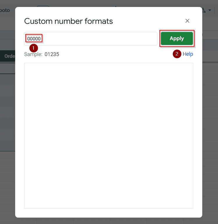
Now, all numbers in that column will be displayed as five digits. The underlying values remain unchanged (e.g., 23), but they’ll appear as 00023 on the sheet. This is great for printing or sharing clean records.
This method is beneficial for creating invoices, customer IDs, or anything that benefits from a uniform format.
How to Format Numbers as Currency on Google Sheets
When working with financial data like sales, costs, or prices, the numbers must look like actual money, not just plain digits. Formatting numbers as currency adds dollar signs, commas, and decimal points, making your sheet easier to read and more professional.
Steps:
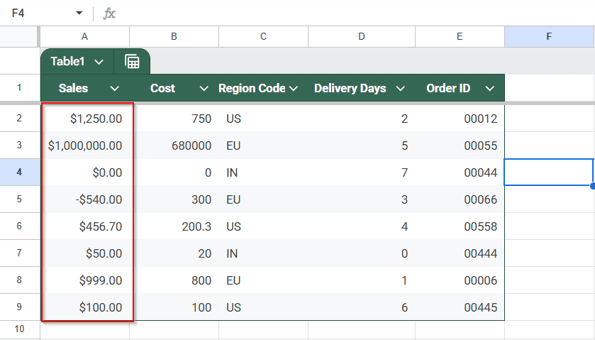
➤ Select your Sales or Cost column (e.g., Column A or B).
➤ Go to Format >> Number >> Custom number format.
➤ Enter: $#,##0.00
➤ Click Apply.

This turns 1250 into $1,250.00 and keeps cents even if they’re .00.
Highlight Negative Numbers in Red and Add Parentheses on Google Sheets
In financial reports, negative values (like losses or expenses) are often shown in red and wrapped in parentheses instead of using a minus sign. This style makes negative numbers stand out and improves readability, especially when reviewing profit and loss figures.
Steps:
➤ Highlight the column that has both positive and negative values (like Sales).
➤ Go to Format >> Number >> Custom number format.

➤ Enter: #,##0.00;[Red](#,##0.00)
➤ Click Apply.
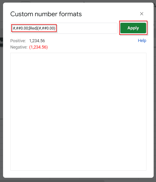
Now, -540 will display as (540.00) in red, while 456.7 stays normal.
Add Units Like “days” or “kg” to Numbers on Google Sheets
If your data involves measurements such as delivery times, weights, or distances, you might want to display units (e.g., “days” or “kg”) directly next to the numbers. Google Sheets lets you do this without changing the actual value by applying a custom number format that adds static text beside each number.
Steps:
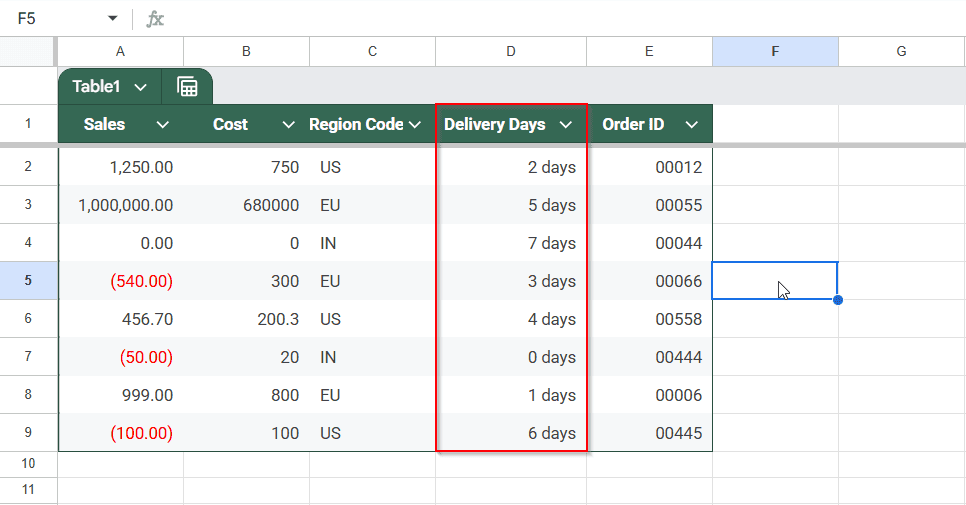
➤ Select your Delivery Days column (Column D).
➤ Go to Format >> Number >> Custom number format.
➤ Enter: 0 “days”
➤ Click Apply.
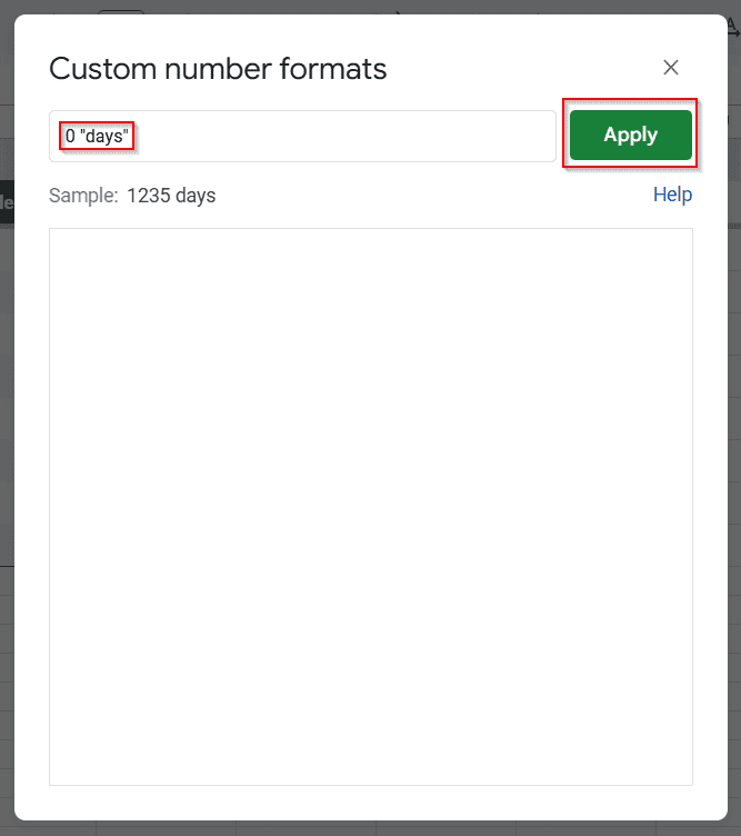
Now, the number 3 becomes 3 days without changing the actual value.
Abbreviate Large Numbers with K, M, B on Google Sheets with the ARRAYFORMULA Function
When working with large values, like sales figures in the thousands or millions, showing the full number can take up space and make your sheet harder to scan. You can simplify this using an ARRAYFORMULA function that shortens large numbers with suffixes like K (thousand), M (million), or B (billion), while keeping the actual value intact.
Steps:
➤ Add a new column next to your Sales column (e.g., Column B)
➤ In cell B2, enter the following formula:
=ARRAYFORMULA(IF(A2:A=””, “”, IF(A2:A>=1000000000, ROUND(A2:A/1000000000,1)&”B”, IF(A2:A>=1000000, ROUND(A2:A/1000000,1)&”M”, IF(A2:A>=1000, ROUND(A2:A/1000,1)&”K”, A2:A)))))
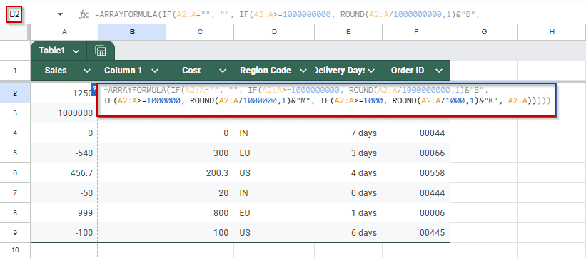
➤ Press Enter. The formula will automatically apply to all rows with data in Column A
➤ The full numbers will now appear shortened in Column B:
- 1250 becomes 3K
- 1000000 becomes 1M
- 999 remains as 999
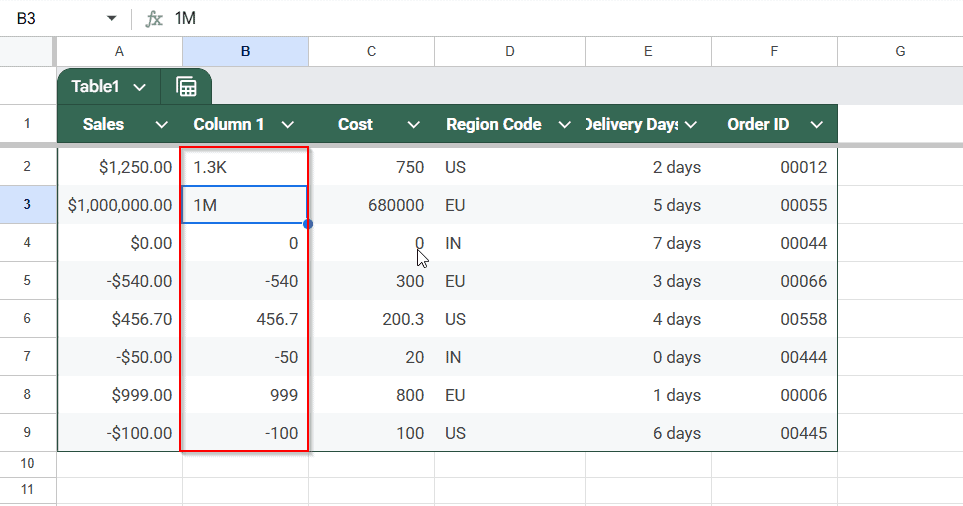
This is a formula-based approach, not a number format, but it gives you the exact same result, without needing any manual formatting. You can use this output column for display purposes while keeping the raw numbers intact for calculations.
Replace Zeros with “N/A” in a Cell on Google Sheet
By default, Google Sheets displays a 0 when a cell contains a zero value. But in many situations, such as cost reports, delivery tracking, or attendance logs, a 0 might be confusing or misleading. To make your data more intuitive, you can use a custom number format that replaces any 0 with “N/A” while keeping other numbers unchanged.
Steps:
➤ Select a column where some values are 0 (like Sales or Cost).

➤ Go to Format >> Number >> Custom number format.

➤ Enter: 0;0;”N/A”
➤ Click Apply.
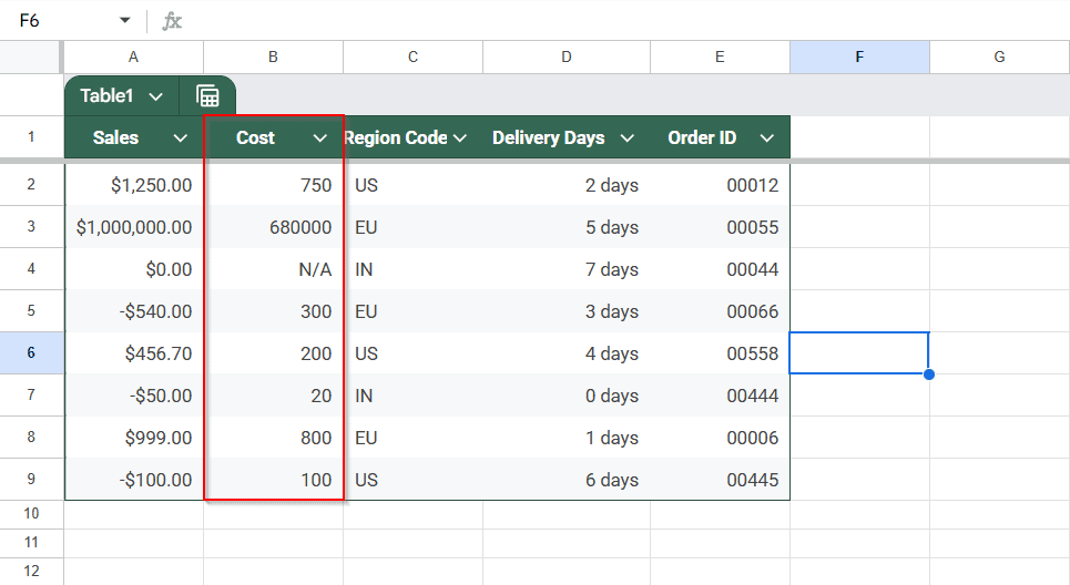
This will show 0 as N/A, while all other values remain unchanged.
Display Text Based on Value (e.g. High, Low)
If you want your sheet to show labels like “High,” “Low,” or “Okay” based on a number’s value, you can use custom number formats without changing the actual number in the cell. This is helpful for performance ratings, score tracking, or any data where you want to give context at a glance.
Steps:
➤ Select your target column.

➤ Go to Format >> Number >> Custom number format.
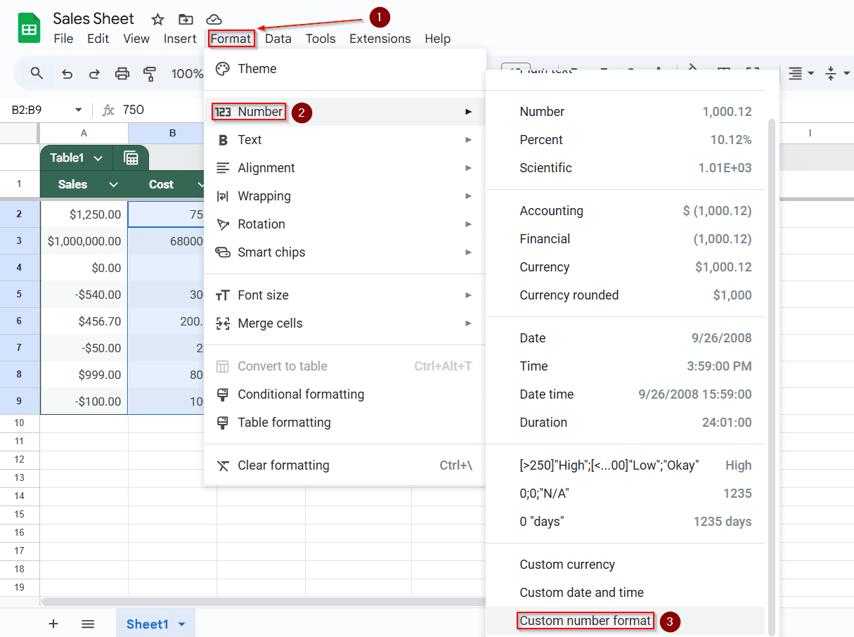
➤ Enter: [>250]”High”;[<100]”Low”;”Okay”
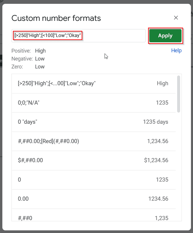
➤ Click Apply.
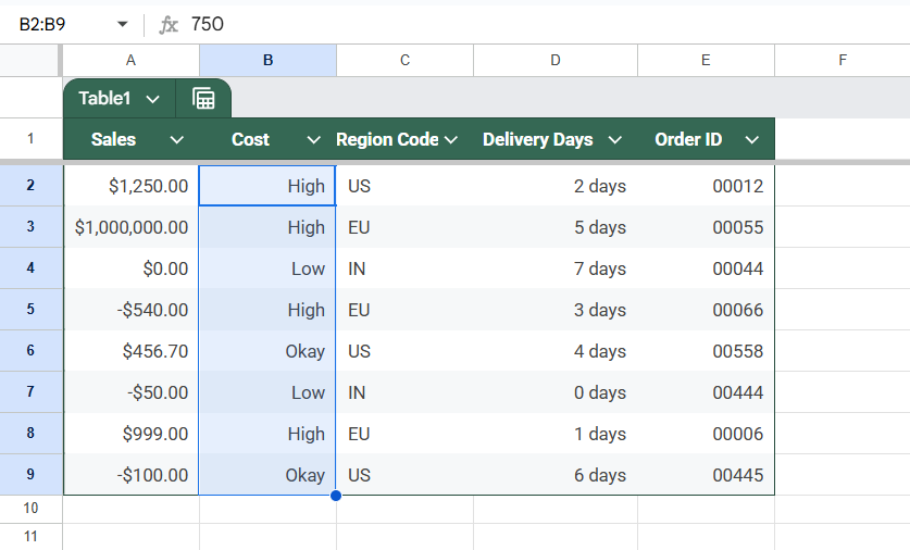
If the value is 300, it will show as “High”; 0 will be “Low”; 100 is “Okay”.
Frequently Asked Questions
How do I create a custom number format in Google Sheets?
➤ Select the cells you wish to format,
➤ Navigate to Format >> Number >> Custom number format.
➤ Enter your desired format pattern in the dialog box and
➤ Click Apply.
This allows you to define how numbers are displayed without altering their actual values.
Can I apply custom formats to dates and currencies?
Yes, Google Sheets supports custom formats for dates, times, and currencies. You can specify exact display formats, including incorporating text and symbols, to enhance clarity and presentation.
How can I display text labels like “High” or “Low” based on numeric values?
Use conditional custom number formats. For example: [>100]”High”;[=100]”Okay”;”Low”
This format displays “High” for values over 100, “Okay” for 100, and “Low” for values below 100.
Can I add colors to differentiate numbers in custom formats?
Yes, you can include color codes in your custom formats. For instance: [Red]#,##0;[Blue]-#,##0;[Green]”Zero”;[Magenta]@
This format displays positive numbers in red, negative numbers in blue, zeros in green, and text in magenta.
Wrapping Up
Custom number formats let you display data clean and smartly, whether you’re tracking budgets, sales numbers, region codes, or delivery times. You can format text, add labels, highlight values, and simplify large numbers without changing your real data.
Experiment with these formats to save time and make your sheets easier to understand. Start with built-in presets and then try the custom formats above to make your spreadsheet truly yours.