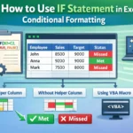
When working with large datasets in Excel, manually checking for differences or matches between two columns can be tedious. Luckily, Excel offers visual tools like Conditional Formatting that make it easier to highlight values that are either the same or different. Whether you’re comparing names, product codes, or dates, this approach helps you instantly spot inconsistencies without scrolling through row by row.
In this article, we’ll guide you through straightforward methods to compare two columns, from quick built-in options to advanced techniques using custom formulas. Each method is designed to save time and improve accuracy,no complex steps involved.
Steps to Highlight Matching Values Between Two Columns:
➤ Select the first column.
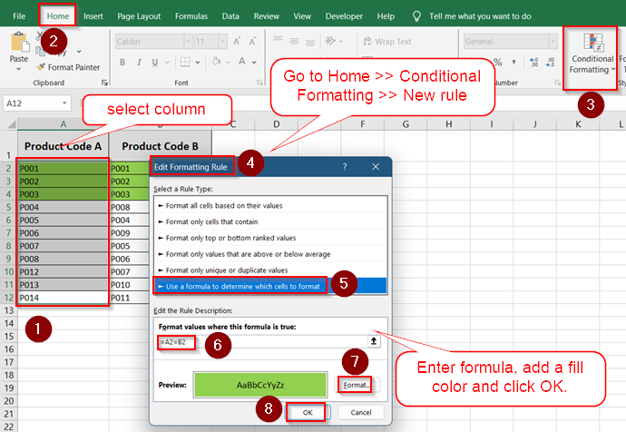
➤ Go to Home >> Conditional Formatting >> New Rule.
➤ Choose Use a formula to determine which cells to format.
➤ Enter the formula: =A1=B1.
➤ Set a format color and click OK.
How Does Conditional Formatting Work Between Two Columns in Excel
Conditional Formatting is an Excel feature that automatically changes the appearance of cells based on the conditions you define. When applied between two columns, it becomes an effective tool for visual comparison. It allows you to spot duplicates, identify mismatches row by row, and highlight any exceptions or inconsistencies across your data, all without writing extra formulas or applying filters.
For instance, if you’re working with two lists of employee names from different departments, Conditional Formatting can instantly color the matching entries or draw attention to differences. This makes it easier to scan through large datasets and catch errors or overlaps at a glance, saving you both time and effort during data reviews.
Use the COUNTIF Function to Highlight Duplicates in Excel
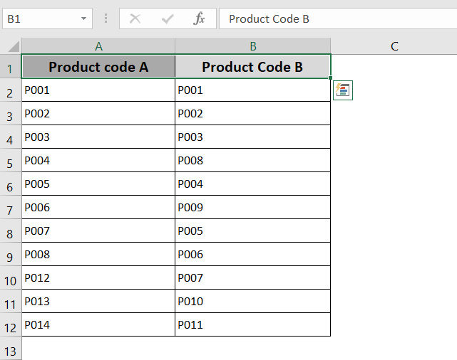
The COUNTIF function is a flexible way to compare two columns by checking if values in one column appear anywhere in the other. This method is useful when rows don’t perfectly align your data, and you want to quickly highlight duplicates or unique entries between the lists.
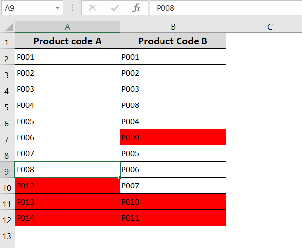
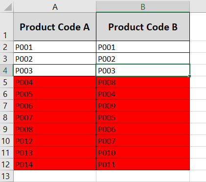
In this example, imagine comparing two lists of product codes from different suppliers. Using Conditional Formatting with COUNTIF lets you visually identify matches and exceptions across the entire column without extra steps.
Steps:
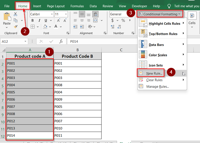
➤ Select the first column range (A2:A12).
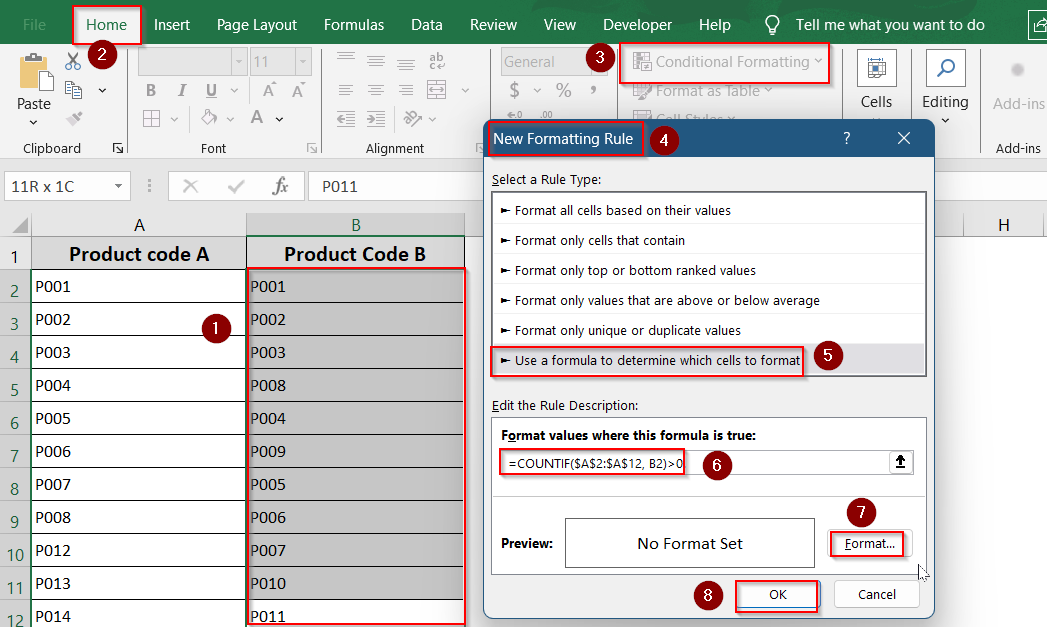
➤ Go to Home tab >> Conditional Formatting >> New Rule.

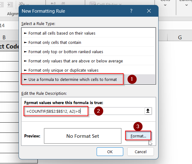
➤ Choose “Use a formula to determine which cells to format.”
For Matching Values
➤ Enter the formula:
=COUNTIF($B$2:$B$12, A2)>0
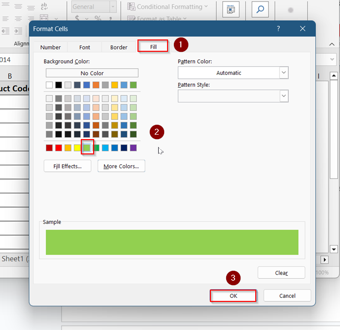
➤ Click Format.
➤Pick a fill color (e.g., green), and click OK.
➤ Repeat for the second column (e.g., B2:B12) using:
=COUNTIF($A$2:$A$12, B2)>0
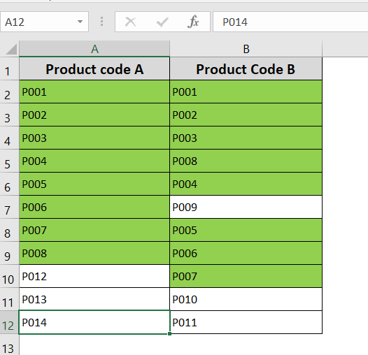
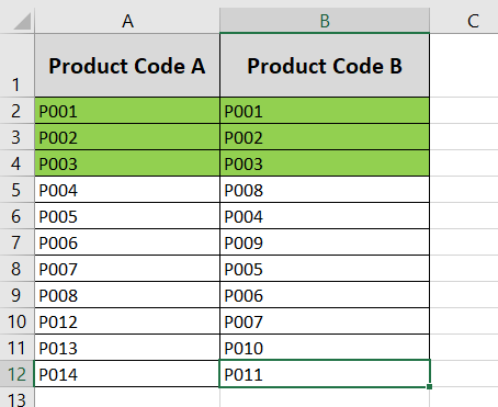
Now, matching product codes will be highlighted in green.
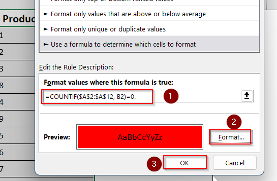
For Unique (Non-Matching) Values
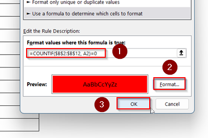
➤ Enter the formula:
=COUNTIF($B$2:$B$12, A2)=0
➤ Click Format, pick a fill color (e.g., red), and click OK.
➤ Repeat for the second column (e.g., B2:B12) using:
=COUNTIF($A$2:$A$12, B2)=0
Now, matching product codes will be highlighted in red, making it easy to compare the two lists visually.
Apply ‘Equal To’ Operator to Compare Row-by-Row in Excel
When comparing data that should align row by row, simple formulas like equal-to (=) and not equal-to (<>) can be beneficial. These formulas enable conditional formatting to highlight cells where values either match exactly or differ in the same row across two columns. This method is ideal for verifying paired lists, matching IDs, or checking data consistency where order matters.
Using conditional formatting with these formulas provides instant visual feedback, making it easier to spot discrepancies or confirm accuracy without manually scanning the data. This straightforward approach saves time and reduces errors when reviewing data that must correspond row-wise.
Steps:
➤ Select the first column range (A2:A12).
➤ Go to Home tab >> Conditional Formatting >> New Rule.
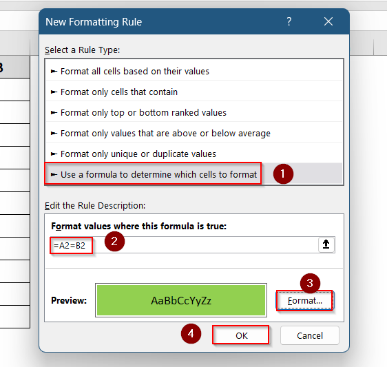
➤ Choose “Use a formula to determine which cells to format.”
For Matching Values
➤ Enter the formula:
=A2=B2
➤ Repeat for the second column (e.g., B2:B12) using:
=B2=A2
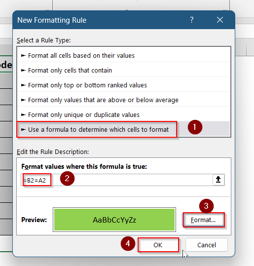
Matching cells are now visible in green.
For Unique (Non-Matching) Values
➤ Enter the formula:
=A2<>B2
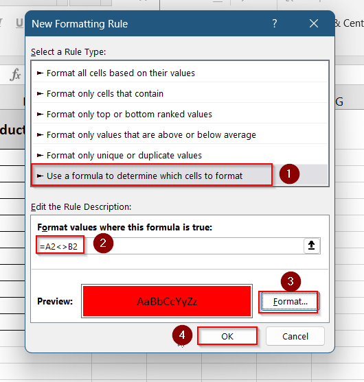
➤ Repeat for the second column (e.g., B2:B12) using:
=B2<>A2
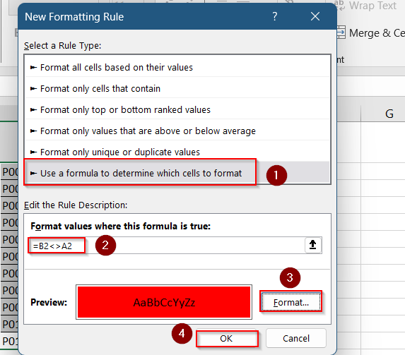
Unique values are now displayed in red.
Frequently Asked Questions
How do I compare two columns for case-sensitive matches using Conditional Formatting?
To perform a case-sensitive comparison between two columns, use the =EXACT(A2, B2) formula inside the Conditional Formatting rule. This function checks whether the text in both cells is exactly the same, including uppercase and lowercase letters. It’s useful when differences in capitalization matter for your dataset.
Can I compare columns across different sheets?
Yes, you can compare columns from different sheets using Conditional Formatting.
➤ In your formula, include the sheet name like this: =A2=Sheet2!B2.
➤ Ensure both sheets exist in the workbook and have aligned data ranges so that Excel can accurately evaluate row-by-row comparisons.
How do I remove conditional formatting later?
If you want to remove Conditional Formatting rules from your worksheet, go to the Home tab, click on Conditional Formatting, and choose Clear Rules. Depending on your needs, you’ll then have the option to remove formatting from either the selected cells or the entire worksheet.
What if my columns have different lengths?
When your columns have different lengths, Conditional Formatting still works row by row but only within the selected range. To avoid errors or partial highlights, apply the rule only to the overlapping portion of both columns where data is present in each corresponding row.
Wrapping up
In this tutorial, we learned how to use conditional formatting to compare two columns in Excel. We explored how to highlight both matching and unique values using the COUNTIF function, and how to compare data row by row with equal-to and not equal formulas.
Whether your data is unordered or lined up row-wise, these techniques make differences and similarities easier to spot. Feel free to download the practice file and share your thoughts and suggestions.