When you’re working with large spreadsheets, it’s easy to lose track of changes between two Excel sheets. Whether you’re reviewing sales records, inventory reports, or updated entries from collaborators, finding differences quickly is critical.
In this article, you’ll learn multiple ways to compare two sheets and highlight differences using Excel’s built-in tools, formulas, and even a simple macro. These methods work for both simple and large datasets whether the differences are in values, formatting, or structure.
Steps to compare two excel sheets:
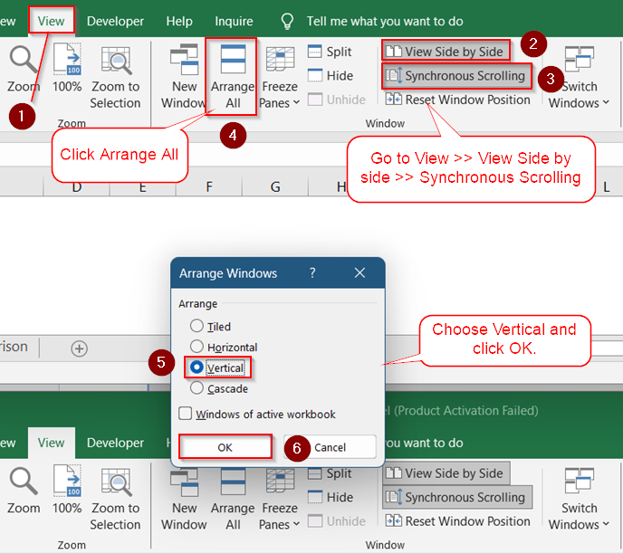
➤ Go to View tab >> Click View Side by Side.
➤ Check Synchronous Scrolling to scroll both sheets together.
➤ Use Arrange All >> choose “Vertical” for better alignment.
➤ Click OK.
What Does Comparing Excel Sheets and Highlighting Differences Mean?
Comparing Excel sheets and highlighting differences means checking two datasets side by side and marking where they do not match. This can involve differences in cell values, formulas, formats, or even missing entries.
For example, if you’re comparing a product list from two different months, highlighting the differences can help you quickly identify what was added, removed, or changed. Excel offers several ways to automate this process visually, so you don’t have to manually check every cell.
View Side by Side Comparison
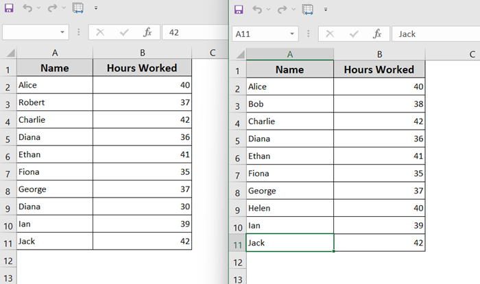
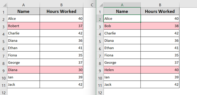
This method is ideal if you want a quick, manual way to scan and compare two Excel sheets without formulas or complex setup. It allows you to place both sheets next to each other, scroll them simultaneously, and visually inspect differences.
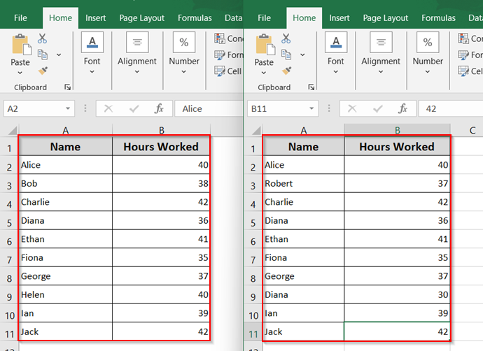
In this example, we’re comparing employee hours in two monthly reports with a list of names and hours worked. This method helps you quickly spot changes like adjustments in total hours or new entries.
Steps:
➤ Open both Excel files (or same file in two windows).
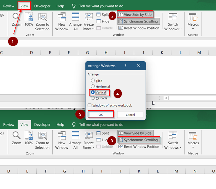
➤ Go to View tab >> Click View Side by Side.
➤ Check Synchronous Scrolling to scroll both sheets together.
➤ Use Arrange All >> choose “Vertical” for better alignment.
➤ Click OK.
This method is best for quick manual reviews.
Highlight Cell Differences Using Conditional Formatting
If you want Excel to automatically highlight cells that differ between two sheets, Conditional Formatting is a smart choice. It uses a simple formula to compare each cell in Sheet1 with the same cell in Sheet2, and visually marks any mismatches.
This method works well when both sheets share the same structure and row alignment, making it perfect for comparing columns like hours worked, prices, or status updates.
Steps:
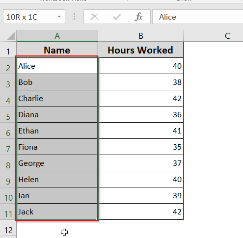
➤ Select range on Sheet1 (e.g., A2:B11).
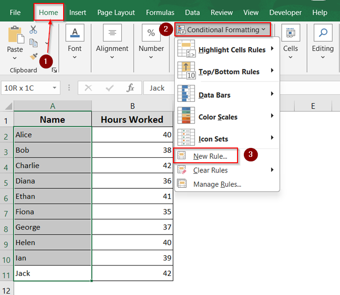
➤ Go to Home >> Conditional Formatting >> New Rule.
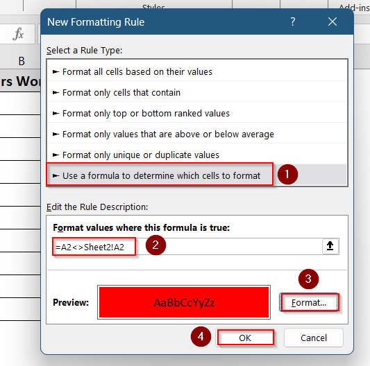
➤ Choose “Use a formula to determine which cells to format“.
➤ Enter formula:
=A2<>Sheet2!A2
➤ Go to Format and add a fill color.
➤ Click OK.
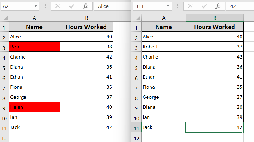
Now highlighted cells are marked in red in Sheet 1 that differ from Sheet 2.
Use a Formula to Compare and Report Differences
Want a clean, text-based summary that clearly states what changed and where? This method uses a custom formula to compare two cells and print the differences in a third sheet.
It’s helpful when you want a separate, readable list of mismatches rather than visual highlights on the original sheets. The formula displays both values side-by-side when there’s a mismatch.
Steps:
➤ Create a new sheet named “Comparison“.
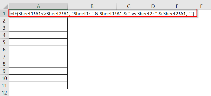
➤ In cell A2, enter:
=IF(Sheet1!A1<>Sheet2!A1, “Sheet1: ” & Sheet1!A1 & ” vs Sheet2: ” & Sheet2!A1, “”)
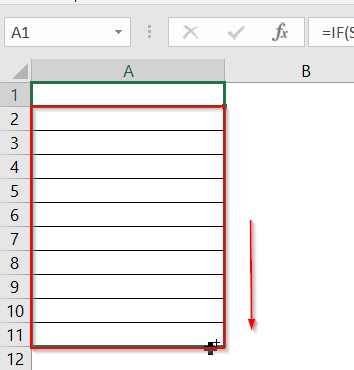
➤ Drag the formula across and down to cover the data range.
Outputs clear text clearly show mismatches between the sheets.

Use Excel’s Inquire Add-In
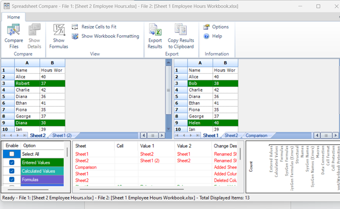
If you’re using Microsoft 365 or Excel Professional Plus, the Inquire add-in is a built-in feature that generates a detailed comparison report between two workbooks.
It highlights differences in formulas, values, cell formats, and more in a side-by-side summary, ideal for auditors or version control. The results are presented in a comprehensive report that’s easy to review.
Steps:
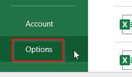
➤ Go to File.
➤ Select Options at the bottom corner.
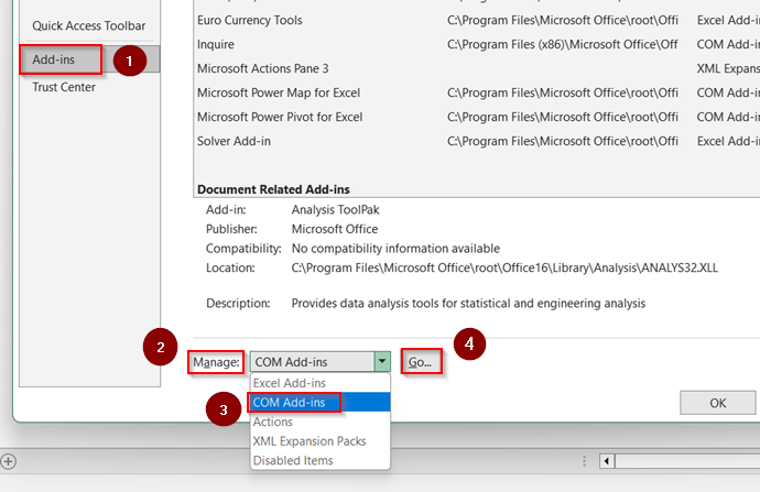
➤ Choose Add-ins >> Manage COM Add-ins >> Go.
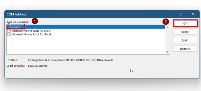
➤ Check Inquire and click OK.
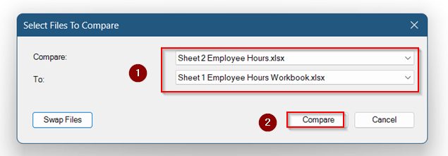
➤ Open Inquire tab in Ribbon >> Click Compare Files.
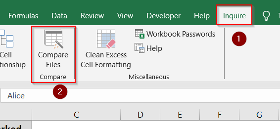
➤ Select both workbooks and click OK.
Now you can review detailed comparisons in a separate report.
Highlight Differences with VBA
For maximum flexibility, a VBA macro can automate the entire comparison process and highlight all mismatched cells across two sheets.
This method is especially useful when dealing with large datasets or when you want to customize how differences are highlighted. All it takes is a simple script you can reuse anytime.
Steps:
➤ Press Alt + F11 to open the VBA Editor.
➤ Insert new Module >> Paste comparison macro script:
Sub HighlightDifferences()
    Dim ws1 As Worksheet, ws2 As Worksheet
    Dim r1 As Range, r2 As Range
    Dim cell1 As Range, cell2 As Range
    Dim diffColor As Long
    Dim maxRow As Long, maxCol As Long
    Dim i As Long, j As Long
    ' Set your worksheets
    Set ws1 = ThisWorkbook.Sheets("Sheet1")
    Set ws2 = ThisWorkbook.Sheets("Sheet2")
    ' Set highlight color
    diffColor = RGB(255, 199, 206) ' light red
    ' Determine max used range
    maxRow = Application.WorksheetFunction.Max(ws1.UsedRange.Rows.Count, ws2.UsedRange.Rows.Count)
    maxCol = Application.WorksheetFunction.Max(ws1.UsedRange.Columns.Count, ws2.UsedRange.Columns.Count)
    ' Loop through each cell to compare
    For i = 1 To maxRow
        For j = 1 To maxCol
            Set cell1 = ws1.Cells(i, j)
            Set cell2 = ws2.Cells(i, j)
            If cell1.Value <> cell2.Value Then
                cell1.Interior.Color = diffColor
                cell2.Interior.Color = diffColor
            End If
        Next j
    Next i
    MsgBox "Comparison complete. Differences highlighted in both sheets.", vbInformation
End Sub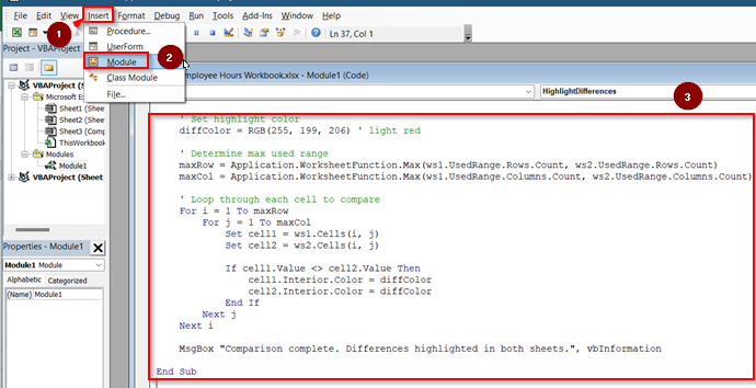
➤Click Run >> Run Sub/Userform to highlight differences.
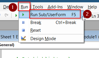
Your results will now be visible in both sheets.
Frequently Asked Questions
Can I compare sheets with different sizes or layouts?
Yes, but the accuracy of formulas depends on consistent cell alignment. If layouts differ, consider using VBA, or Inquire for more flexible comparison based on values rather than positions.
How do I remove highlights after comparison?
To remove highlights, go to Home >> Conditional Formatting >> Clear Rules >> choose “Clear Rules from Selected Cells” or “Entire Sheet“. This removes only the formatting, not your original data.
Can I compare values but ignore formatting differences?
Yes, Conditional formatting and formulas only compare actual cell values not cell colors, borders, or fonts. To include formatting in the comparison, use the Inquire add-in.
Can I highlight only the rows that contain any mismatch?
Yes, you can adjust your conditional formatting formula to check entire rows and apply a format if any value differs across that row. Alternatively, use VBA to flag full rows instead of individual cells.
Wrapping up
In this tutorial, we learned how to compare two Excel sheets and highlight differences using various techniques. We covered simple Side by Side viewing, Conditional Formatting, custom formulas, the Inquire add-in, and a VBA macro to automate cell-by-cell comparison. Feel free to download the practice file and share your thoughts and suggestions.