Flipping data vertically in Excel means reversing the order of rows from top to bottom. This is useful when you’re working with lists or tables that need to be reordered, such as timelines, sorted names, or historical records. Excel doesn’t have a direct “flip” feature, but there are multiple ways to achieve the same result using formulas, helper columns, Power Query, or VBA.
In this article, we’ll cover every practical method to flip data vertically whether you prefer manual tools, formulas, or automation. We’ll also share a sample dataset so you can follow along step-by-step.
Steps to flip data vertically in Excel using Sort By function:
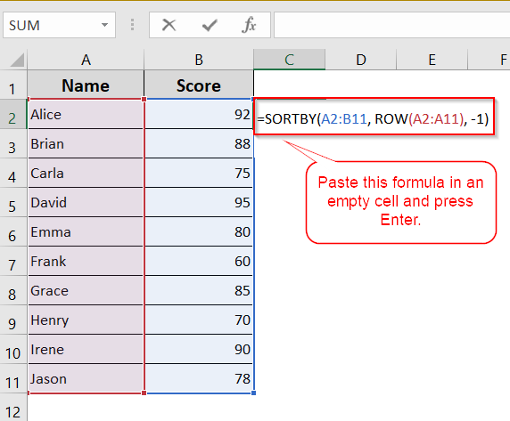
➤ Select a blank area to output the flipped data.
➤ Use this formula: =SORTBY(A2:B11, ROW(A2:A11), -1)
➤ Press Enter.
What Does "Flipping Data Vertically" Mean in Excel?
Flipping data vertically in Excel means reversing the order of your rows so that the bottom-most row moves to the top and the top-most row shifts to the bottom. This can be useful when you need to invert a timeline, reverse a list of entries, or prepare data in a different sequence for analysis or presentation.
Excel doesn’t provide a direct “flip” command, but you can achieve vertical flipping using a variety of methods such as helper columns with sorting, Excel formulas, Power Query, or VBA macros. Each method suits different needs depending on whether you want a one-time flip or a dynamic solution that updates automatically.
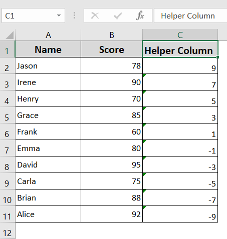
Sort Using Helper Column
This is the easiest and most reliable method if you’re using older versions of Excel or if you want a manual approach. It’s perfect for beginners and doesn’t require complex formulas or tools. You’ll simply assign reverse-order numbers to each row and use Excel’s Sort feature to flip the data.
Steps:
➤ Insert a new column (e.g., Helper column) to the right or left of your dataset.
➤ In the first row of the helper column (e.g., C2 cell) , type the formula:
=COUNTA(B2:B11)+1-ROW()
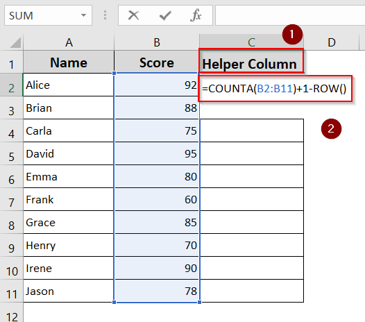
➤ Drag the formula down to apply it to all rows.
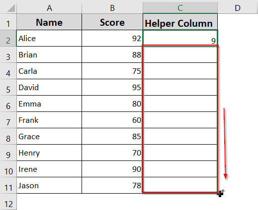
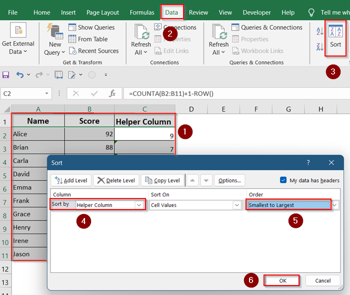
➤ Select your entire dataset including the helper column.
➤ Go to the Data tab >> Click Sort.
➤ Sort by the helper column in Smallest to Largest order.
Your data is now flipped vertically. You can delete the helper column if needed.
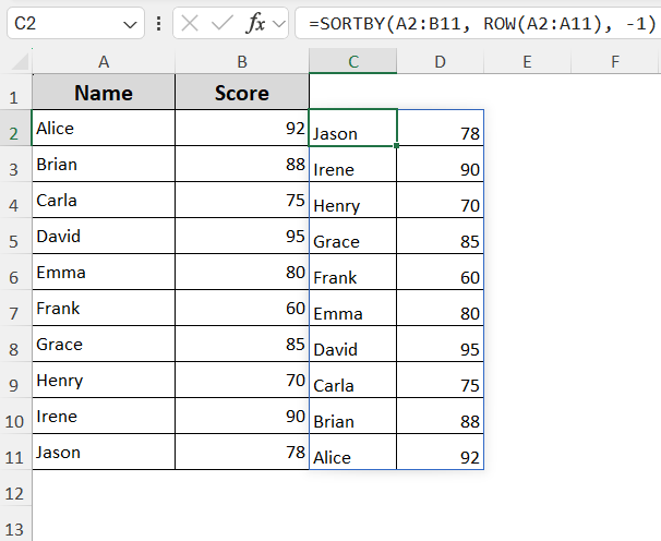
Apply SORT By Function (For Excel 365 and Excel 2019+)
If you’re using a modern version of Excel, this is the cleanest and most dynamic method. It allows you to reverse rows without modifying the original data or adding any helper columns. Moreover, it updates automatically if your original data changes without extra columns.
Steps:
➤ Select a blank area to output the flipped data.
➤ Use this formula:
=SORTBY(A2:B11, ROW(A2:A11), -1)
➤ Press Enter.
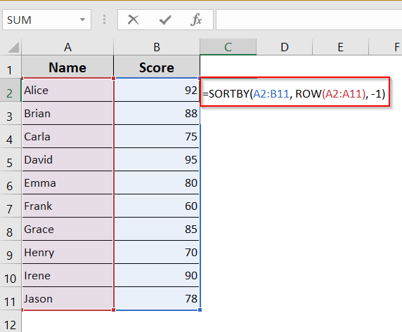
Now, Excel will return a vertically flipped version of your table.
Use Power Query (Advanced but Powerful)
Power Query is a built-in data transformation tool in Excel that gives you full control over data manipulation. It’s ideal for recurring tasks and offers a clean interface for transforming datasets. This method is best suited for intermediate to advanced users or anyone dealing with larger datasets.
Steps:
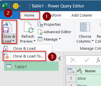
➤ Select your dataset >> Go to Data tab >> Click From Table/Range.
➤ In Power Query Editor, go to Transform >> Click Reverse Rows.
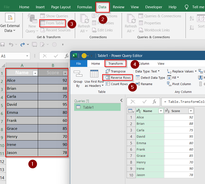
➤ Click Close & Load to send the flipped data back into Excel.
Now, your flipped data will appear in a new worksheet.

Flip Data Using VBA Macro
If you’re comfortable with VBA, a simple macro can flip your data vertically with a single click. This is great if you want to automate the process.
Steps:
➤ Press Alt + F11 to open the VBA Editor.
➤ Insert a new module and paste this code:
Sub FlipRowsVertically_ColsAandB_KeepHeader()
    Dim ws As Worksheet
    Dim lastRow As Long
    Dim i As Long
    Dim tempA As Variant, tempB As Variant
    Set ws = ActiveSheet
    lastRow = ws.Cells(ws.Rows.Count, "A").End(xlUp).Row
    For i = 2 To (lastRow + 2) \ 2 ' Start from row 2
        ' Swap values in Column A
        tempA = ws.Cells(i, "A").Value
        ws.Cells(i, "A").Value = ws.Cells(lastRow - i + 2, "A").Value
        ws.Cells(lastRow - i + 2, "A").Value = tempA
        ' Swap values in Column B
        tempB = ws.Cells(i, "B").Value
        ws.Cells(i, "B").Value = ws.Cells(lastRow - i + 2, "B").Value
        ws.Cells(lastRow - i + 2, "B").Value = tempB
    Next i
End Sub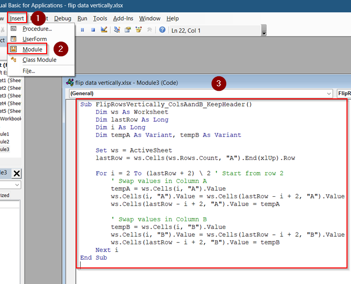
➤ Run the macro and Close the editor.
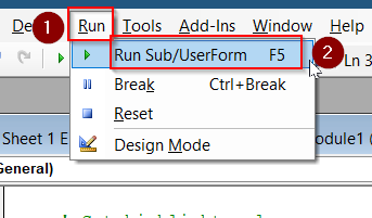
Now the results will be visible in your Excel sheet.
Frequently Asked Questions
Can I flip data without flipping the header?
Yes, just exclude the header row when applying the flip. In VBA, start from Row 2 instead of Row 1. Power Query also lets you preserve headers by treating them as column names, not data.
What if my data has blanks?
Blank rows or cells stay in place relative to their position, they just move with the rest of the data. None of the methods fill in or skip blanks automatically, so your structure remains intact.
Does Power Query flip into a new sheet?
Yes, it loads the flipped data into a new sheet by default, formatted as a table. This method keeps your original sheet safe and lets you keep both versions if needed.
Can I flip and transpose at once?
Not directly. You’ll need to transpose first (using Paste Special), then flip the transposed data using a method from this article.
Wrapping Up
In this tutorial, we learned multiple ways to flip data vertically in Excel. We covered helper columns with sorting, Power Query transformations, and VBA automation. Each method is suited for different user levels from beginner to advanced. Feel free to download the practice file and share your thoughts and suggestions.