When analyzing spreadsheets, it’s often useful to visually identify when one value exceeds another such as highlighting profits that beat projections or scores that surpass benchmarks. Fortunately, Excel allows you to do this easily using Conditional Formatting.
In this article, you’ll learn different ways to highlight a cell if its value is greater than the one in another cell. These methods work with both adjacent and non-adjacent cells and don’t require complex formulas or VBA.
Steps to highlight a cell with greater value using Conditional Formatting:
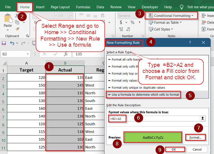
➤ Select the range you want to compare.
➤ Go to Home >> Conditional Formatting >> New Rule >> Use a formula.
➤ Type =B2>A2 and choose a Fill color from Format.
➤Click OK.
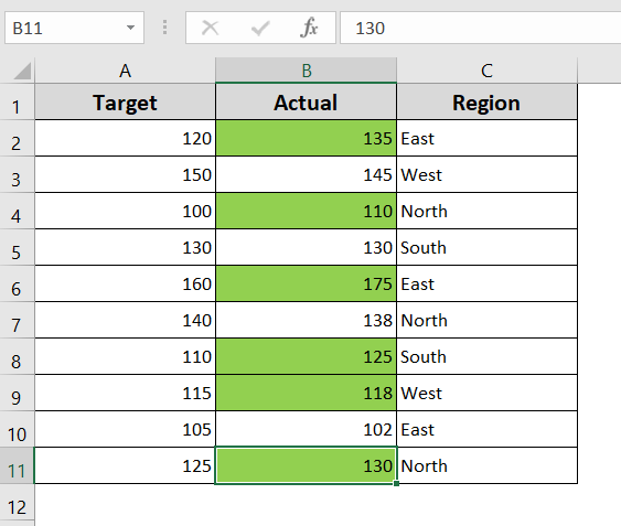
Compare Two Columns Row by Row
If you have two side-by-side columns (e.g., Target and Actual), and you want to highlight cells in Column B when the value is greater than the same-row value in Column A, this method is perfect.
Steps:
➤ Select the range where comparison should happen (e.g. B2:B11).
➤ Go to Home >> Conditional Formatting >> New Rule.
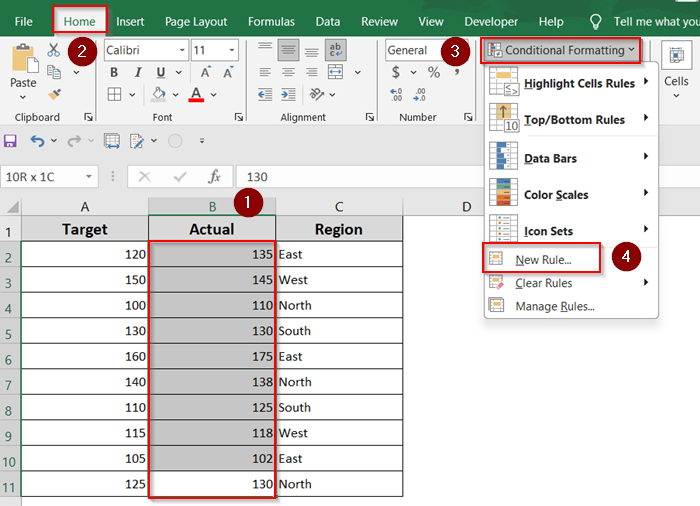
➤ Choose Use a formula to determine which cells to format.
➤ Enter this formula:
=B2>A2.
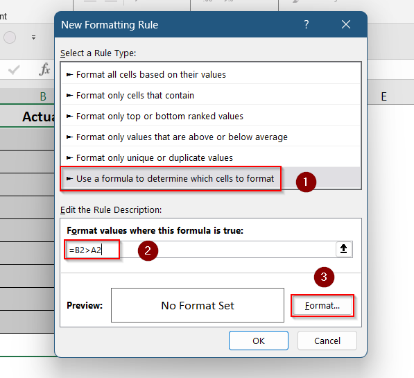
➤ Click Format >> Fill, choose your highlight color (like light green), then click OK.

Every cell in Column B that has a greater value than its corresponding cell in Column A will now be highlighted.
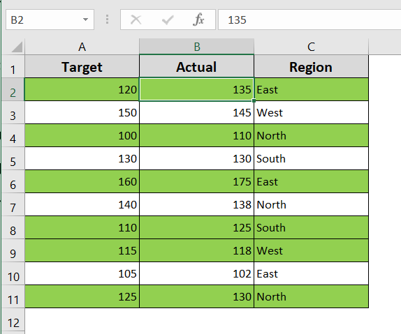
Highlight Entire Row If One Cell Is Greater Than Another
This method highlights the entire row when a specific value in one column is greater than a value in another column on the same row. This is helpful when you want the full row to stand out for easier review.
Steps:
➤ Select the full range of rows you want to format (e.g., A2:C11).
➤ Go to Conditional Formatting >> New Rule >> Use a formula to determine…
➤ Enter this formula:
=$B2>$A2
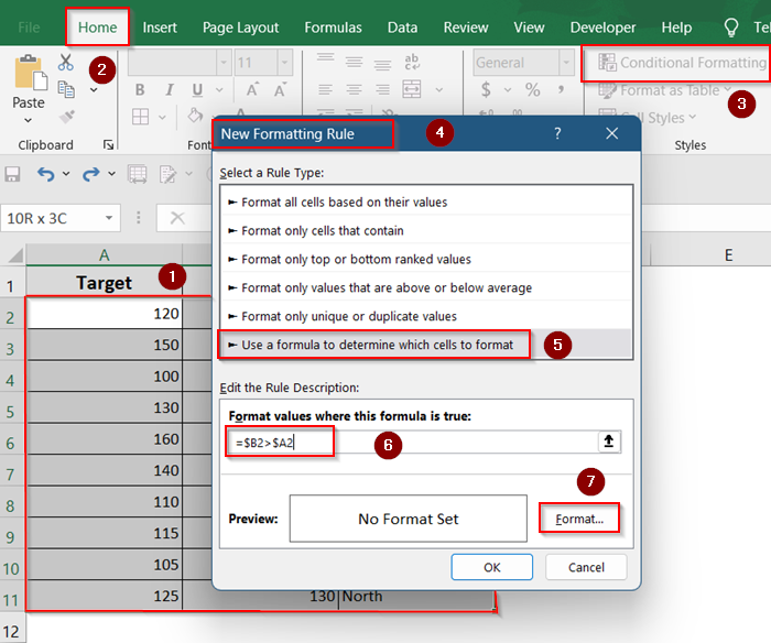
➤ Apply a Fill color from the Format menu and press OK.

Now, if the value in Column B is greater than the value in Column A, the entire row will be colored.
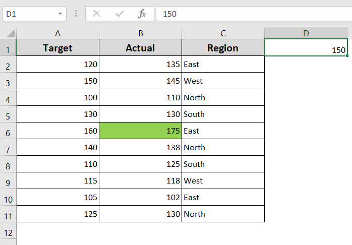
Highlight If Greater Than a Fixed Cell
In some cases, you might want to compare each value against a fixed benchmark cell (e.g., B2 > D1). This method allows comparisons against a static reference point instead of comparing row by row.
Steps:
➤ Select the range you want to format, such as B2:B11.
➤ Add your desired value (e.g., 150) in cell D1 to compare.
➤ Go to Home >> Conditional Formatting >> New Rule.
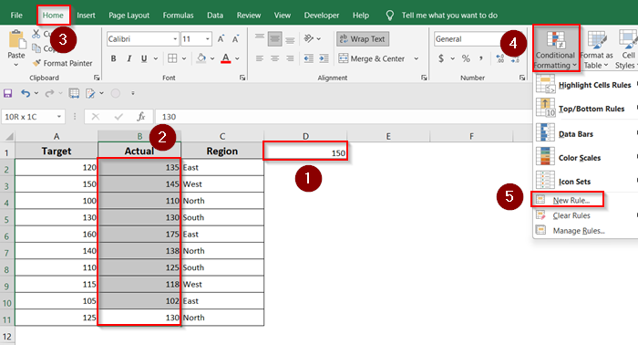
➤ Choose Use a formula to determine which cells to format.
➤ Enter this formula:
=B2>$D$1
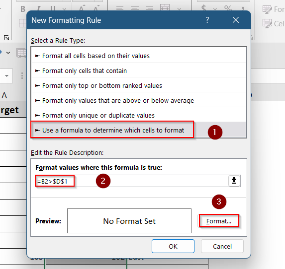
➤ Choose your desired Fill color from Format and click OK.
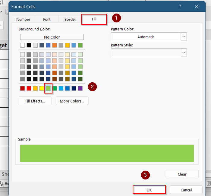
All values greater than the fixed cell (D1) will be highlighted, regardless of row position.
Use Built-in “Greater Than” Rule for Static Comparisons
For straightforward comparisons against a constant value, Excel’s built-in “Greater Than” rule offers a quick solution.
Steps:
➤ Select the range you wish to format (e.g. B2:B11).
➤ Go to Home >> Conditional Formatting >> Highlight Cell Rules >> Greater Than…
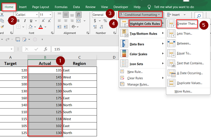
➤ Enter the value to compare against (e.g., 120).
➤ Choose a formatting style and click OK.
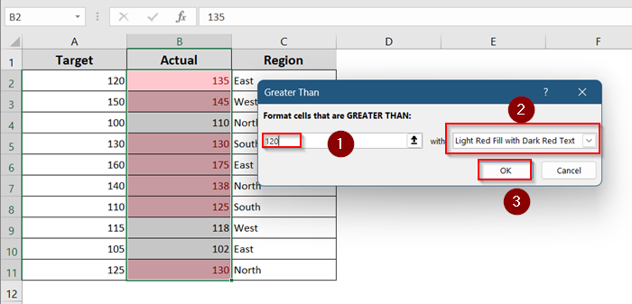
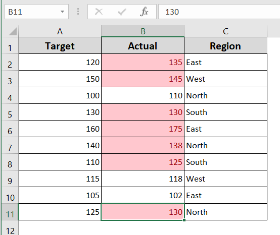
Cells with values greater than the specified number will be highlighted accordingly.
Frequently Asked Questions
Does this work for text values too?
No, this method works best with numeric values. Text comparison using greater than (>) will not yield meaningful results unless you’re doing alphabetical comparisons, which is rarely practical for conditional formatting.
Will the formatting update if I change the values?
Yes. Conditional formatting in Excel is dynamic. If you adjust any value in the range or reference cell, the formatting will instantly update based on the new comparison result, no need to reapply the rule.
Can I apply this rule across different worksheets?
Not directly. Conditional formatting can’t refer to cells on a different worksheet using the formula method. To apply similar logic, you’d need to copy the reference values to the same sheet or use helper columns within the same sheet.
Wrapping Up
In this tutorial, you explored multiple ways to highlight cells in Excel when one value is greater than another, from simple Conditional Formatting rules to custom formulas and even row-based highlights. These methods are perfect for budget sheets, score comparisons, and any dataset that involves cell-to-cell evaluation. Feel free to download the practice file and share your thoughts and suggestions.