The equation of a trendline is the closest relation between variables. To find the equation of a trendline in Excel, we can use the built-in feature or we can calculate it manually.
An equation is helpful to find out the future or non-existent values. It is also helpful to summarize complex data. To make better decisions based on predictions, equations of trendlines also come in handy.
To find the equation of a trendline in Excel,
➤ Plot a chart.
➤ Go to Chart Elements >> Trendline >> Select the trendline type.
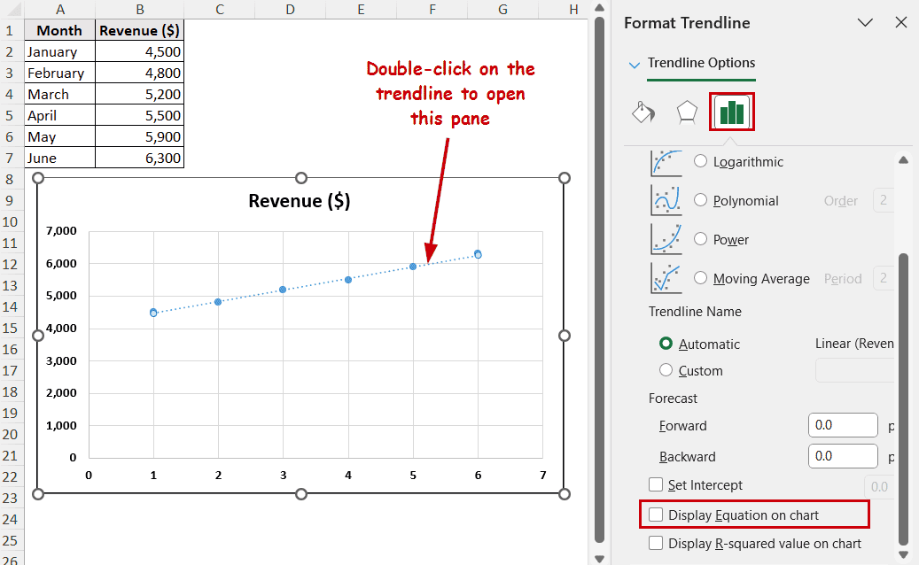
➤ Double-click on the trendline to open the Format Trendline Pane.
➤ Check Display Equation on chart.
In this tutorial, we will go through how to find the equation of a trendline in Excel. To display the equation directly on the chart, we can use the equation feature of charts. To manually find out the coefficients of the trendline formula, we need to use different Excel functions.
Download Practice WorkbookFind Equation Automatically on Chart
Excel has the Display Equation on chart option available to insert an equation in a chart directly.
The equation will be the best fit or close to the actual relation between the data from the source. Excel determines this equation solely based on your selected trendline type (linear, polynomial, exponential, etc.).
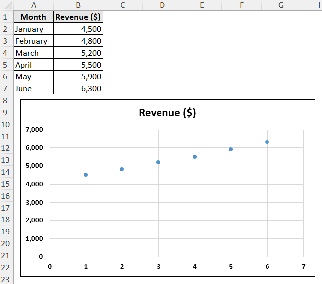
Suppose we have monthly revenue data and a scatter plot illustrating the data.
Here’s how you can add a trendline, find the equation of the trendline, and display the trendline’s equation on the chart:
Steps:
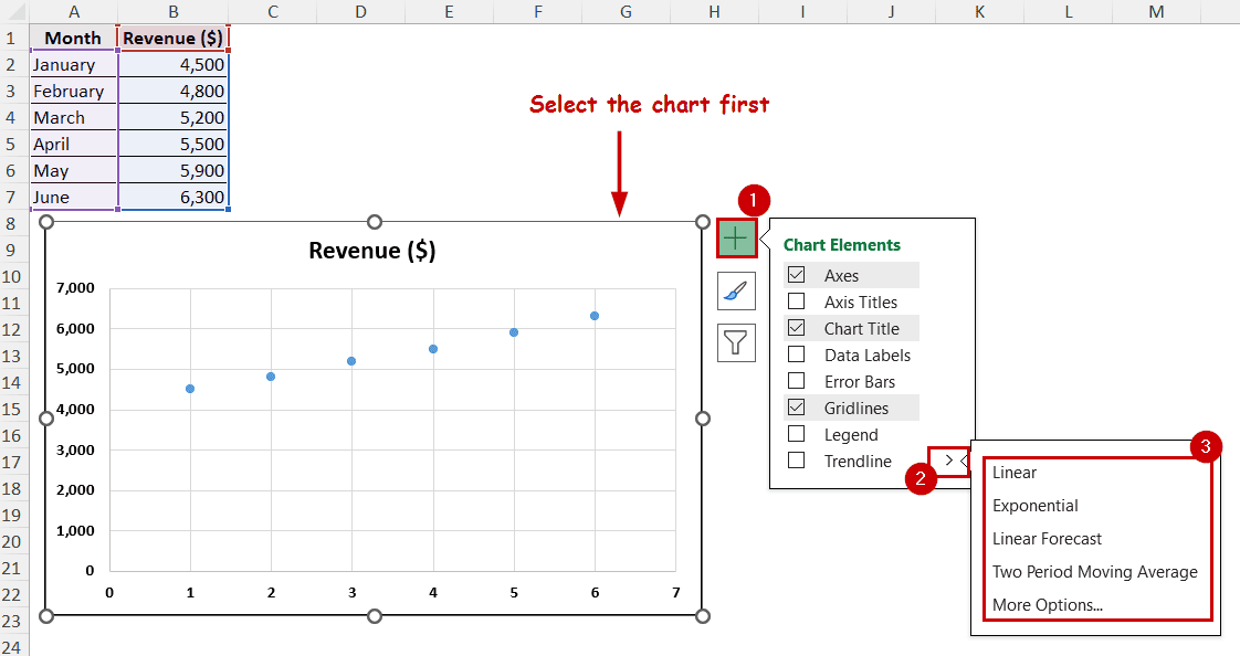
➤ Select the chart.
➤ Go to Chart Elements >> Trendline >> select the type of trendline.
➤ Now double-click on the trendline to open the Format Trendline pane.
➤ In the pane, check Display Equation on chart under Trendline Options.
➤ Move the equation to the desired position of the chart.

You will have the trendline equation displayed on the chart.
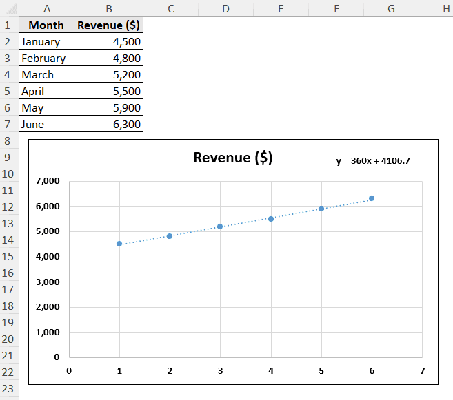
The x here is the month values (January = 1, February = 2, etc.), and y indicates the revenue. The relation indicates the revenue increases by $360 each month, with a $4106 surplus from the start.
Detailed Calculations of Each Type of Trendline
Different types of trendlines (linear, exponential, etc.) have different mathematical formulas. Coefficients in these formulas represent different things on the graph. Excel has different functions, which we can use directly or combine them to represent those points.
You can use these methods to find the equations without plotting the chart.
Linear Trendline Formula
Linear lines represent the equation: y=mx+c. Here, m is the slope of the trendline, and c is the value where the trendline crosses the Y-axis. Excel has SLOPE and INTERCEPT functions to determine this value.
Steps:
➤ Select a cell (B9) and type the following formula for slope:
=SLOPE(B2:B7,A2:A7)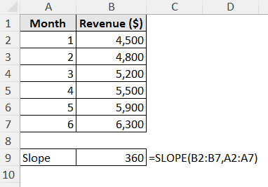
➤ Use the following formula for intercept:
=INTERCEPT(B2:B7,A2:A7)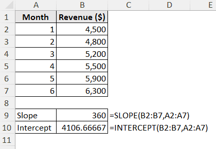
360 and 4106 are the same values we got from the equation earlier.
Exponential Trendline Formula
Exponential trendline equations follow the formula: y=aebx. Here a and b are constants that can be determined with the help of EXP, INDEX, LINEST, and LN functions.
Steps:
➤ Select an output cell (B9) and insert the following formula:
=EXP(INDEX(LINEST(LN(B2:B7),A2:A7),1,2))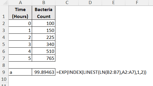
This is the “a” value. Change B2:B7 with y values and A2:A7 with x values.
➤ Select an output cell (B10) and insert the following formula for the “b” value:
=INDEX(LINEST(LN(B2:B7),A2:A7),1)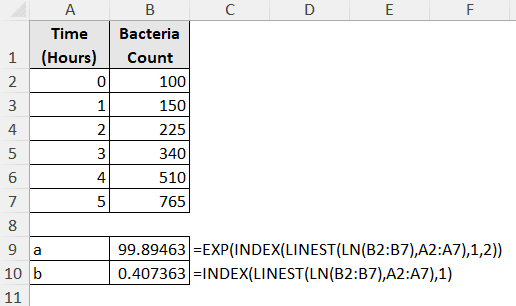
Swap B2:B7 with y and A2:A7 with x values.
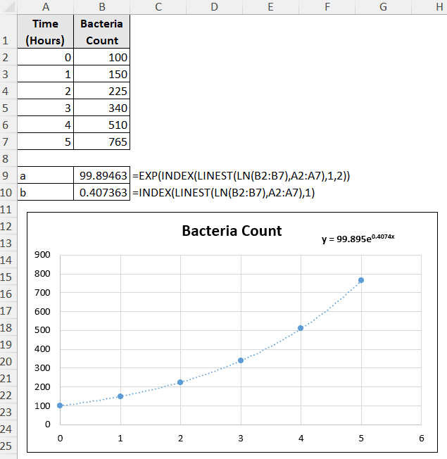
These are the same values if we use the equation feature of Excel.
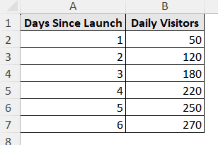
Logarithmic Trendline Formula
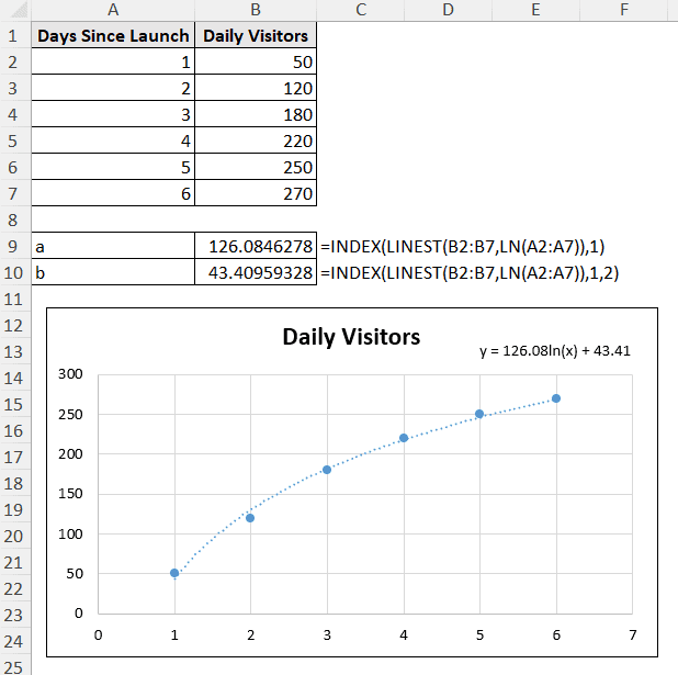
The logarithmic equation is: y=a*ln(x)+b. We need to use INDEX, LINEST, and LN functions to determine the values of a and b. To demonstrate, we are going to use the following dataset. It shows the website traffic growth since the launch of a sample website.
Steps:
➤ Select an output cell(B9) and insert the following formula:
=INDEX(LINEST(B2:B7,LN(A2:A7)),1)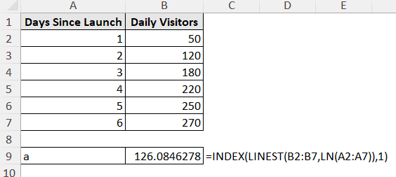
➤ Change B2:B7 with your Y and A2:A7 with your X values.
➤ Insert the following formula in an output cell (B10) for the b value:
=INDEX(LINEST(B2:B7,LN(A2:A7)),1,2)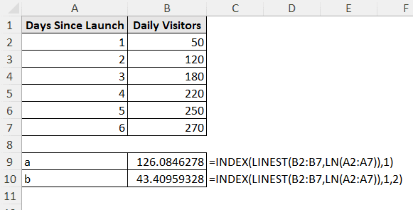
These values resonate with the equation from the chart.
Polynomial Trendline Formula
For polynomials. Excel can go up to the 6th-degree equation. However, we are demonstrating using a degree of 3. This is the equation for a 3rd-degree polynomial equation: y=b3x3+b2x2+b1x+c. The functions needed to find these constants are INDEX and LINEST.
Steps:
➤ Select an output cell (B10) and insert the following formula:
=INDEX(LINEST(B2:B8,A2:A8^{1,2,3}),1)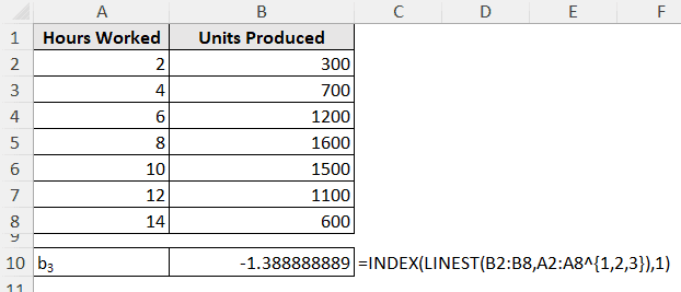
➤ Use the following formula for b2:
=INDEX(LINEST(B2:B8,A2:A8^{1,2,3}),1,2)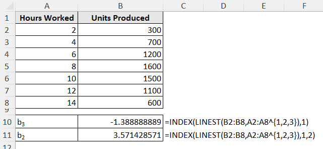
➤ For b1, use the following formula in the output cell (B12):
=INDEX(LINEST(B2:B8,A2:A8^{1,2,3}),1,3)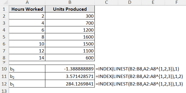
➤ Use the following formula in the output cell (B13) for c:
=INDEX(LINEST(B2:B8,A2:A8^{1,2,3}),1,4)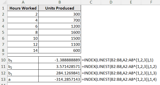
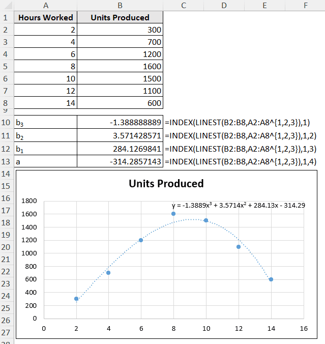
As usual, you can change B2:B8 with your y values and A2:A8 with the x value range. The result is similar to the automatic process.
Suppose you have a second-degree equation: y=b2x2+b1x+c. You need to use this formula for b2:
=INDEX(LINEST(y-range, x-range^{1,2}), 1)
The formula for the value of b1 will be:
=INDEX(LINEST(y-range, x-range^{1,2}), 1)
You can adjust the rest of the constants and even other degree equations similarly.
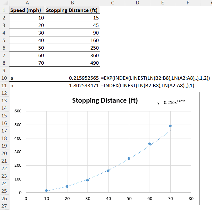
Power Trendline Formula
The “power” trendline follows the formula: y=axb . We need to use a combination of EXP, INDEX, LINEST, and LN functions to determine the values of a and b.
Steps:
➤ Select an output cell (B10) and insert the following formula for a:
=EXP(INDEX(LINEST(LN(B2:B8),LN(A2:A8),,),1,2))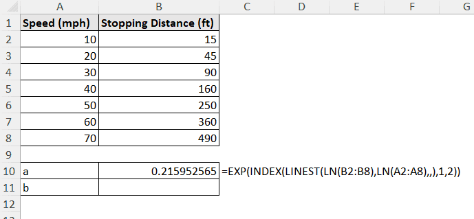
➤ For b, use the following formula in the output cell (B11):
=INDEX(LINEST(LN(B2:B8),LN(A2:A8),,),1)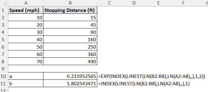
You can change B2:B8 with your y-values’ range and A2:A8 with x-values’ range. The results are similar to the chart’s values.
Note: There is a moving average option for the trendline type in Excel. It’s a smoothing technique, not a mathematical model. That’s why it can’t have an equation like other trendline types.
Issues with Trendline Equations in Excel
- Excel returns an R-squared value based on the transformed data. For example, the R-squared value reflects the fit of ln(y) instead of y in exponential trendlines. So, the data fit appears better than it actually is.
- Logarithmic and exponential trendlines may not always match manual calculations because of internal approximations.
- All x and y values need to be positive for power trendlines.
- Excel ignores hidden/filtered data for charts. These data can create a mismatch with manual calculations.
FAQ
Can I use a trendline equation to forecast future values?
Yes, insert a future or unknown x value in the trendline equation to get the y value for the possible scenario. However, avoid this extrapolation for values that is far beyond the data source. In that case, there is always a risk of inaccuracy.
How to increase decimal places in the trendline equation?
To increase the decimal places in an equation, double-click on the equation to open the Format Trendline Label pane. Under the Label Options, you can find the number format of the equation. You can change the format and decimal places there.
What’s the difference between R-squared value and the equation?
R-squared value represents the fit of the trendline with the data source, 0 being not fit and 1 being the perfect fit. Meanwhile, the equation represents the trendline’s mathematical formula.
Can I use a trendline for non-numeric X-values?
Excel treats non-numeric values as numeric ranks (1, 2, 3, …). For dates, Excel can also count them in different numbers (from January 1st, 1990). So, while you can create a trendline with non-numeric values, it is better not to use equations for these lines.
Concluding Words
In this tutorial, we have covered how to find the equation of a trendline in Excel, both using Excel’s built-in features and formulas. Excel’s Display Equation on chart feature helps to display the equation directly on the chart. To find the coefficients of trendlines’ mathematical equations, we need to use a combination of LINEST, INDEX, LN, and EXP functions.
Feel free to download the practice workbook and let us know about your feedback.