How to Return the Cell Address of a Match in Excel

In Excel, you might often need not just the value from a lookup, but also the exact cell address where that value is found. This is especially useful when you want to reference or highlight that cell dynamically in your formulas or reports. Excel doesn’t have a built-in function that directly returns a cell address from a match, but by combining functions like ADDRESS, ROW, COLUMN, MATCH, CELL, INDEX, and XLOOKUP, you can easily retrieve addresses based on your lookup criteria.

In this article, you’ll learn several practical ways to return a cell address of a match in Excel, including using ADDRESS with MATCH, combining CELL with INDEX or XLOOKUP, and generating addresses for named ranges or specific positions. Let’s get started.

A simple and effective way to return the cell address of a match in Excel is by combining the ADDRESS, ROW, COLUMN, and MATCH functions. This method is useful when you’re searching for a value across a row or column and want to display the exact cell location.

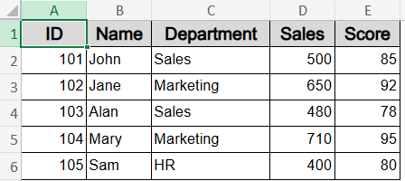
We’ll use a sample dataset where the first row (A1:E1) contains headers like ID, Name, Department, Sales, and Score. Suppose you want to find the address of a header (like “Score”) dynamically:

In this example, we’ll search for a Name in the header row (A1:E1) or any horizontal range, and return the address of the matching cell.

Steps:

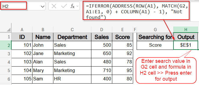
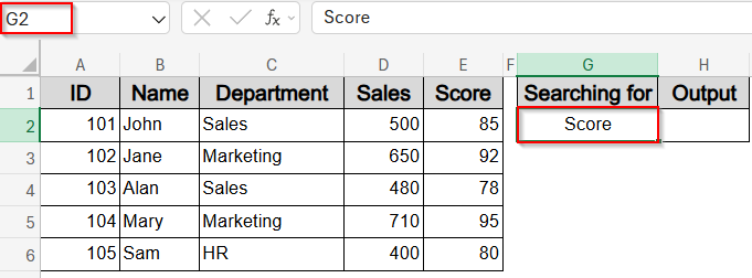
➤ In G2, type the header or value you want to search for (for example, Score).

➤ In H2, enter this formula:

➤ Press Enter.

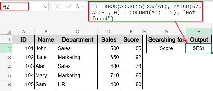
This formula searches for the value in G2 within the range A1:E1. If it finds a match, it returns the cell address, such as $E$1. If no match is found, it displays “Not found”.

This method combines the ADDRESS and MATCH functions to return the cell address of a match found vertically within a column. It’s useful when you want to locate the row position of a specific value in a column and retrieve its exact cell address.

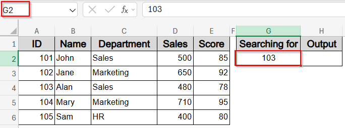
In this example, we’ll search for an ID in the range A2:A6 and return the address of the matching cell in column A.

Steps:

➤ In cell G2, enter the ID you want to find (e.g., 103).

➤ In cell H2, enter this formula:

➤ Press Enter.

The formula finds the row position of the value in G2 within A2:A6 and returns the absolute cell address of the matching ID in column A. For example, if you enter 103 in G2, the formula will return $A$4.

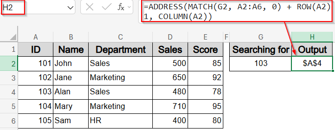
Now you have your exact cell which is A4 based on your search value such as 103.

This method helps you find the full address of a named range in Excel, returning the reference as a text string like $A$1:$E$6. This is useful when you want to display or use the entire range address dynamically in your formulas or reports.

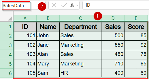
For example, if you have a named range called SalesData referring to the dataset from A1 to E6, this formula will return the full range address $A$1:$E$6.

Steps:

➤ Define your named range SalesData covering your dataset (e.g., A1:E6) using the Name Box beside the Formula Bar.

➤ In any cell where you want to display the full range address such as A9, enter the formula:

➤ Press Enter.

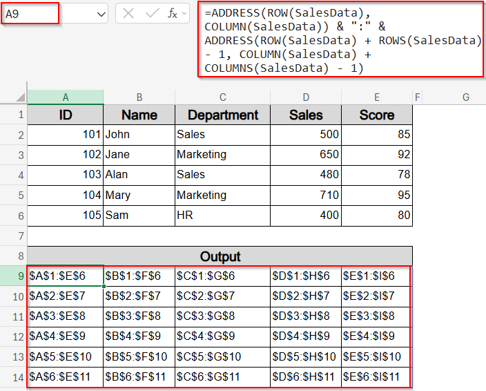
This formula concatenates the address of the first cell in the range with the address of the last cell, creating a full reference string for the named range.

This method combines the CELL, INDEX, and MATCH functions to return the cell address corresponding to a lookup value. It’s useful when you want to find the address of a cell that matches a specific criterion within a dataset.

For example, using our sample dataset, if you search for a Score associated with a particular Name, this formula returns the address of the matching Score cell.

Steps:

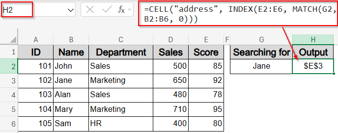
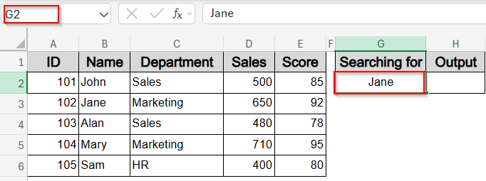
➤ In cell G2, enter the lookup value, for example, a Name like Jane.

➤ In any cell where you want the address to appear such as H2, enter this formula:

➤ Press Enter.

This formula searches the range B2:B6 (Names) for the value in G2 using MATCH, then uses INDEX to return the corresponding cell from the E2:E6 (Scores) column. The CELL and address  function then returns the absolute address of that cell. For example, if G2 is Jane, the formula returns $E$3.

This method uses the CELL function combined with XLOOKUP to return the cell address of a matching value. XLOOKUP searches for a value and returns the corresponding cell reference, which CELL then converts to an address.

For example, using our dataset, if you look up a Name in column B and want to find the cell address of the matching Score in column E, this formula will do that.

Steps:

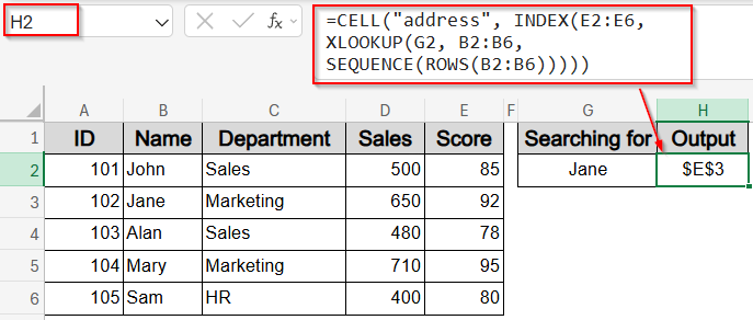
➤ In cell G2, type the lookup Name, for example, Jane.

➤ In any output cell, enter this formula:

➤ Press Enter.

This formula uses XLOOKUP to find the position of G2 in B2:B6 and returns the row number within that range. INDEX then returns the corresponding cell in E2:E6, and CELL(“address”, …) outputs its address. For Jane, the result will be $E$3.

Frequently Asked Questions

How can I retrieve the cell address of a match in Excel?

You can use formula =ADDRESS(ROW(range)+MATCH(value, range, 0)-1, COLUMN(range)) to return the exact cell address where a specific value appears in a defined range, making lookups more informative.

Can I use INDEX and MATCH to find a cell address?

Yes, you can combine INDEX and MATCH with the CELL + address function to return the address of a cell containing a matched value, which is helpful when you want location data instead of content.

How do I find the address of the last cell in a range?

To find the last cell’s address in a rectangular range, use formula: =ADDRESS(ROW(range) + ROWS(range) – 1, COLUMN(range) + COLUMNS(range) – 1). This formula returns the bottom-right cell reference of the selected range.

How can I find the address of a cell with the highest or lowest value?

To find the address of the highest value, use formula: =ADDRESS(MATCH(MAX(range), range, 0) + ROW(range) – 1, COLUMN(range)). Replace MAX with MIN function in the same formula to return the address of the lowest.

Wrapping Up

In this tutorial, we explored multiple practical methods to return the cell address of a match in Excel. Whether you prefer combining ADDRESS with MATCH function, using CELL with INDEX and MATCH function, or using dynamic formulas with named ranges, these techniques help you pinpoint exact cell locations easily. Feel free to download the practice file and share your feedback.