When working with structured datasets in Excel, you may want to calculate the average of values but only when a related cell contains certain text. Whether it’s a product name, region, or category label, Excel’s AVERAGEIF and AVERAGEIFS functions make this possible with just a few steps.
In this article, you’ll learn how to find averages based on cells that contain specific text whether that’s an exact match, a partial match using wildcards, or even multiple conditions using AVERAGEIFS function. We’ll also cover how to use a cell reference instead of hardcoding the criteria.
Steps to find average in Excel if cell contains text:
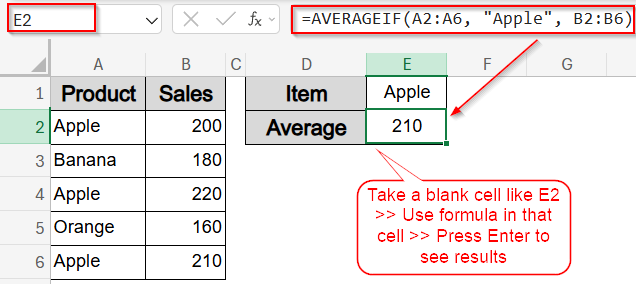
➤ Take an empty cell (e.g., E2),
➤ Use this formula:
=AVERAGEIF(A2:A6, “Apple”, B2:B6)
➤ Press Enter to see output.
Reference a Value Based on Exact Text Match
If your data contains clear, repeated values like “Apple“, this method allows you to average corresponding numeric values in another column using the AVERAGEIF function.
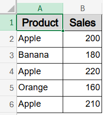
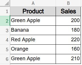
To demonstrate how the AVERAGEIF function works when referencing text, we’ll use a simple dataset of products and their corresponding sales values. This dataset simulates a common scenario where you need to calculate the average sales for a specific product name like “Apple” across multiple rows.
Steps:
➤ In an empty cell (e.g., E2), enter this formula:
=AVERAGEIF(A2:A6, “Apple”, B2:B6)
Change references as needed.
➤ Press Enter to see output.
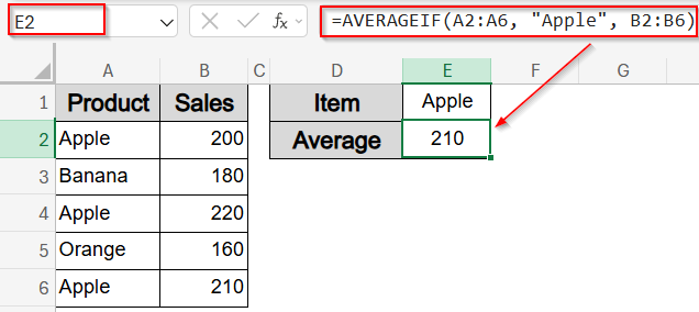
This returns the average of all sales where the product is exactly “Apple“, which in this case is 210 by summing up all values and dividing them by their number.
Reference Text from Another Cell Instead of Typing It
If you want to make the formula dynamic, you can type the text (e.g., “Apple“) in a lookup cell like E2 and refer to that cell in your formula. This makes it easier to change the lookup condition without editing the formula.
Steps:
➤ In cell E1, type the word you want to average, such as Apple.
➤ In a blank cell like E2, use this formula:
=AVERAGEIF(A2:A6, E1, B2:B6)
Change references as needed.
➤ Press Enter to see the results.
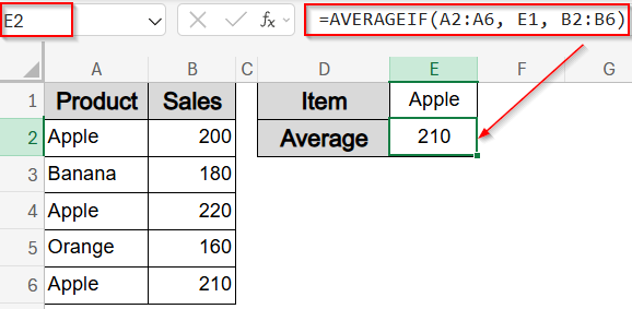
Now you can just change the value in E1 to “Banana” or “Orange” and the average will update automatically.
Use Wildcards to Match If a Cell Contains Partial Text
If your labels aren’t consistent because it contains text like like “Green Apple” or “Red Apple” you can use wildcards like asterisk sign (*) to find partial matches. This method returns the average of values where the keyword appears anywhere within the text, making it perfect for messy datasets.
This is the dataset with variation that we will be using:
Steps:
➤ In a blank cell like E2, use this formula:
=AVERAGEIF(A2:A6, “*Apple*”, B2:B6)
Change references as needed.
➤ Press Enter to see the results.
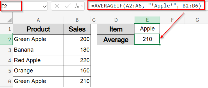
This formula averages sales of all products that include the word “Apple“, even if it’s part of a longer phrase. It matches cells like “Green Apple” and “Red Apple“.
Apply Multiple Text Conditions with AVERAGEIFS Function
Use AVERAGEIFS function when you need to filter by more than one text condition, such as Product and Region. This method returns the average of values that meet all specified criteria, helping you build more refined and targeted summaries in your reports.
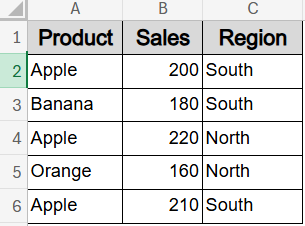
To achieve this, we’ll add a new column called Region in column C which specifies the location such as South or North for each product in our worksheet.
Steps:
➤ In a blank cell like F2, use this formula:
=AVERAGEIFS(C2:C6, A2:A6, “Apple”, B2:B6, “South”)
Change references as needed.
➤ Press Enter to see the results.
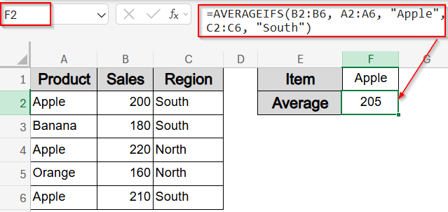
This formula calculates the average sales from column C, where the fruit is “Apple” and the region is “South“. In this case, it averages 200 and 210.
Frequently Asked Questions
What does AVERAGEIF do in Excel?
AVERAGEIF function calculates the average of numbers that meet a single condition in another column. It’s useful when you want to summarize values based on labels like product names, categories, or departments without manually filtering rows.
Can AVERAGEIF check if a cell contains a word?
Yes. By using wildcards like *apple* between asterisks, AVERAGEIF function can detect partial text inside a cell. This helps you average values even when the keyword is part of a longer phrase or label.
What if I want to use more than one condition?
You should use the AVERAGEIFS function. It lets you apply multiple conditions at once like matching both a product and a region which makes it ideal for detailed reporting or layered data filtering in structured datasets.
Can I reference the condition from another cell?
Yes. Instead of typing the condition inside the formula, you can point to a cell like E1. This makes your formulas more flexible and easier to update, especially in interactive sheets or dashboards.
Wrapping Up
In this tutorial, we learned how to use Excel’s AVERAGEIF and AVERAGEIFS functions to find average values if a cell contains text, whether it’s a direct match like “Apple” or a partial string using wildcards. We also explored how to make formulas dynamic by referencing other cells, and how to use multiple criteria for complex filtering. These functions are essential when analyzing text-tagged data like product names, regions, or categories. Feel free to download the practice file and share your feedback.

