In Excel, you may often need to verify whether a cell contains any value from a predefined list of items. This is particularly helpful for validating user inputs, flagging specific content in datasets, or filtering rows based on keywords. While Excel doesn’t offer a built-in function that directly checks if a cell contains any item from a list, you can achieve it using formulas based on SEARCH, ISNUMBER, COUNTIF, XLOOKUP, MATCH, or even array functions in Excel 365.
In this article, we’ll learn every practical way to check if a cell contains text from a list, including combinations with functions like IF, INDEX, dynamic array formulas, and even manual filtering with Find & Select. Let’s get started.
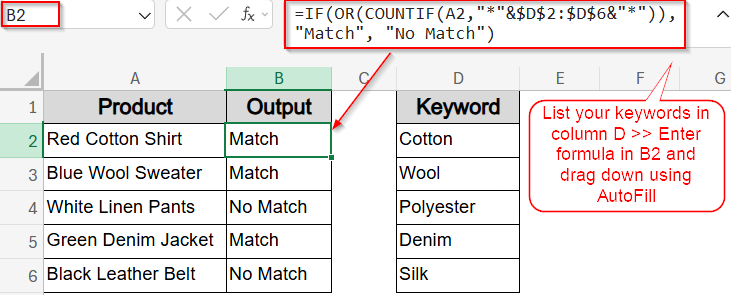
Steps to check if a cell contains text from a list in Excel:
➤ Create Keyword list in column D.
➤ In a blank cell like B2, enter formula:
=IF(OR(COUNTIF(A2,”*”&$D$2:$D$6&”*”)), “Match”, “No Match”)
➤ Press Enter and drag down using the AutoFill handle.
Match Text from a List with SEARCH, ISNUMBER and OR Functions (Excel 365)
This method uses Excel 365’s dynamic arrays to check if any keyword in a list exists within a given cell. It’s efficient for flagging matches using boolean logic.
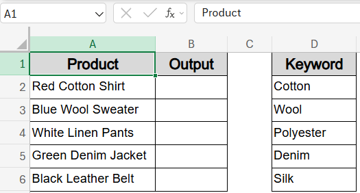
We’ll use a dataset where column A holds product descriptions (e.g., clothing items), and column D lists keywords we want to flag (like Cotton, Wool, Leather, etc.). The formula will go into column B, where it will output TRUE if the description in column A contains any of the listed keywords, and FALSE if it doesn’t.
Steps:
➤ In a blank cell like B2, enter formula:
=OR(ISNUMBER(SEARCH($D$2:$D$6,A2)))
➤ Press Enter and drag down using the AutoFill handle.
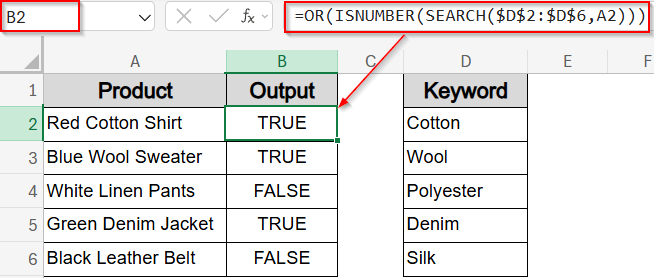
This returns TRUE if any keyword from D2:D8 is found in column A and FALSE if no match is found.
Check for List Matches Using COUNTIF with Wildcards
This method uses the COUNTIF function combined with wildcard characters (*) to check whether any of the keywords in a list appear anywhere within a given text string. Unlike exact match functions, COUNTIF with wildcards allows partial matching, making it ideal for scanning product descriptions or longer text entries. It’s also compatible with older Excel versions and doesn’t require dynamic arrays.
Steps:
➤ In a blank cell like B2, enter formula:
=IF(OR(COUNTIF(A2,”*”&$D$2:$D$6&”*”)), “Match”, “No Match”)
➤ Press Enter and drag down using the AutoFill handle.
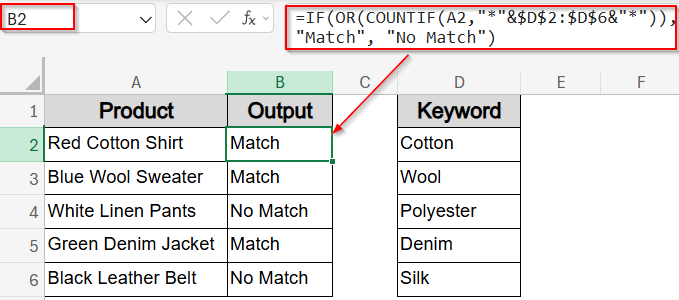
It returns “Match” if column A contains any keyword from the list in column D and “No Match” for vice-versa.
Try SUMPRODUCT with SEARCH and ISNUMBER Functions
This method is ideal when you’re working in older Excel versions that do not support dynamic array formulas like in Excel 365. It uses the SEARCH function to check for the presence of any keyword from a list within a text string, ISNUMBER function to confirm matches, and SUMPRODUCT function to aggregate the results. This method returns TRUE if at least one keyword is found and FALSE otherwise.
Steps:
➤ In a blank cell like B2, enter formula:
=SUMPRODUCT(–ISNUMBER(SEARCH($D$2:$D$6, A2)))>0
➤ Press Enter and drag down using the AutoFill handle.
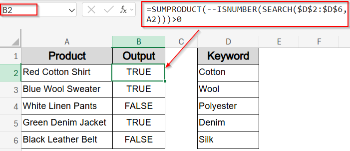
This returns TRUE if at least one keyword from D2:D6 is found within the text in column A; otherwise, it returns FALSE.
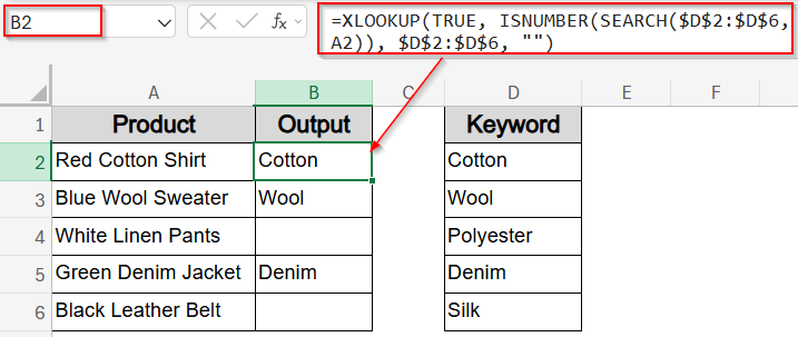
Extract Matching List Using XLOOKUP with SEARCH or COUNTIF Functions
This method is ideal when you want to not only check for the presence of a keyword from a list but also return the actual matched keyword. By combining XLOOKUP function with either SEARCH or COUNTIF function, you can scan the cell for multiple possible matches and return the first one found. This method works especially well in Excel 365 and 2021.
Steps:
➤ In a blank cell like B2, enter formula:
=XLOOKUP(TRUE, ISNUMBER(SEARCH($D$2:$D$6, A2)), $D$2:$D$6, “”)
➤ Alternatively, you can also use this formula with COUNTIF function:
=XLOOKUP(1, COUNTIF(A2, “*” & $D$2:$D$6 & “*”), $D$2:$D$6, “”)
➤ Press Ctrl + Shift + Enter for older Excel versions and only Enter for newer Excel versions.
➤ Drag down using the AutoFill handle.
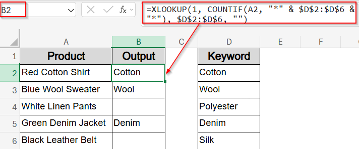
This returns the first keyword from D2:D6 found in each cell from column A, or blank if none match.
Apply INDEX with MATCH and SEARCH Functions to Return First Match
For Excel versions that don’t support XLOOKUP function, you can replicate similar results using INDEX and MATCH function with an array formula. This will return the first keyword found from the list in the output of each cell.
Steps:
➤ In a blank cell like B2, enter formula:
=IFERROR(INDEX($D$2:$D$6, MATCH(1, SEARCH($D$2:$D$6, A2)^0, 0)), “”)
➤ Press Enter and drag down using the AutoFill handle.
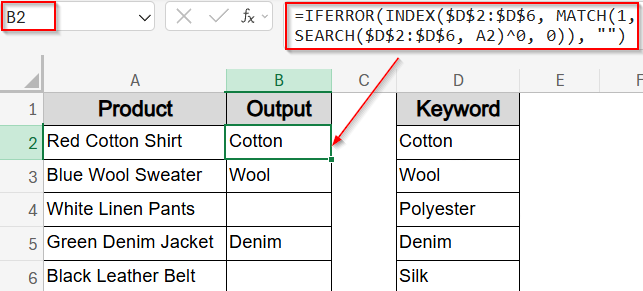
This returns the first keyword from D2:D6 found in each cell from column A, or blank if none match.
Manual Check Using Find & Select Feature
If you prefer a manual approach without formulas, Excel’s Find & Select feature can help you quickly identify whether a cell contains a keyword from your list. It will display all matches found altogether with cell references. Although not automated, this helps quickly explore datasets without formulas.
Steps:
➤ Press Ctrl + F to open the Find dialog box.
➤ In the Find what box, type the keyword (e.g., “Cotton“).
➤ Click Search Options drop-down, set Within to Sheet or Workbook.
➤ Click Find All to see every match.
➤ Repeat this process for other keywords in your list as needed.
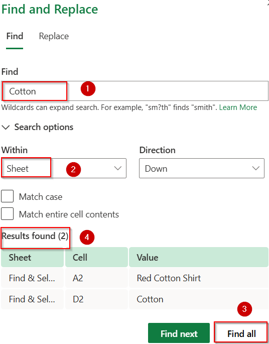
We found matches for Cotton in A2 and D2 cells based on our results.
Frequently Asked Questions
How do I check if a cell contains any text from a list in Excel?
You can use formula =OR(ISNUMBER(SEARCH(list_range, cell))) or COUNTIF function with wildcards to scan for keywords. These formulas return TRUE if any list item appears within the text.
Can I extract the matched keyword instead of just checking?
Yes. Use functions like XLOOKUP or INDEX + MATCH with SEARCH to return the first keyword that appears in the cell. These formulas help extract rather than only verify a match.
What happens if no keyword is found in a cell?
If no match is found, formulas like IFERROR function or logic-based IF statements can return a blank or custom label like “No Match” to handle such cases cleanly without showing errors.
Are these formulas compatible with Excel 2013 or older versions?
Yes, methods with SUMPRODUCT, COUNTIF, and INDEX/MATCH function are compatible with older Excel versions and do not require dynamic array support or modern functions like XLOOKUP.
Can I use these formulas inside Conditional Formatting rules?
Yes. You can insert SEARCH, COUNTIF, or ISNUMBER logic directly into Conditional Formatting to visually flag rows or cells that match your list criteria without needing extra columns.
Wrapping Up
In this tutorial, we explored all practical ways to check if a cell contains text from a list in Excel. From basic logic checks using SEARCH, COUNTIF, and ISNUMBER function to dynamic extractions with XLOOKUP, INDEX, and MATCH function, each method offers a unique benefit based on your Excel version and use case. Feel free to download the practice file and share your feedback.