Ranking data is a crucial part of analyzing performance, whether you’re working with exam results, employee metrics, or product sales. It helps you identify top performers, compare values quickly, and create leaderboard-style reports. While Excel doesn’t offer a built-in “Rank and Sort” button, it gives you all the tools needed to build flexible, powerful ranking systems using formulas and dynamic arrays.
In this article, you’ll learn several practical methods to rank data in Excel using sorting functions like SORT, TAKE, RANK, COUNTIF, INDEX, and MATCH. Whether you’re building a dashboard or filtering top entries, these techniques will help you rank your data clearly and automatically.
Steps to rank data in excel with sorting:
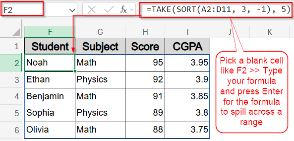
➤ In a blank cell like F2, type this formula:
=TAKE(SORT(A2:D11, 3, -1), 5)
Here, you can change 5 to represent top X values of your preference.
➤ Press Enter for the formula to spill.
Sort and Rank Scores Using SORT and RANK Functions
To display student scores in descending order along with their rank, use the SORT and RANK functions together. This method helps organize your dataset visually while clearly showing who performed best. Using our dataset, we’ll sort scores from Noah (95) to Mia (75) in column A and assign each student their rank based on the Score column.
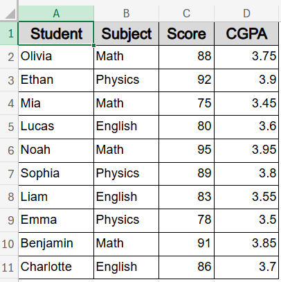
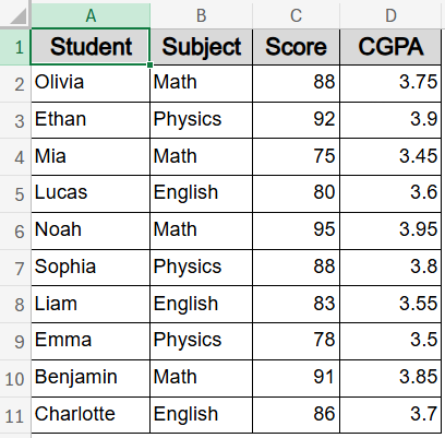
We’ll use a sample dataset containing the names, subjects, scores, and CGPAs of 10 students to demonstrate ranking data in Excel with sorting.
Steps:
➤ In cell F2, enter this formula to sort by score (column C):
=SORT(A2:D11, 3, -1, FALSE)
Here, A2:D11 is the dataset, 3 refers to the Score column, and -1 sorts it in descending order.
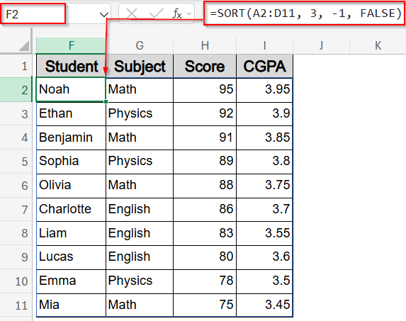
This formula spills your sorted data immediately from column F to I.
➤ In J2, enter this formula to rank the sorted scores:
=RANK(C2, $C$2:$C$11, 0)
Here, C2 is the score being ranked, $C$2:$C$11 is the full score range, and 0 ranks from highest to lowest.
➤ Drag it down to J11.
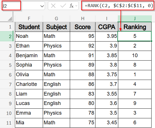
Now we have a sorted table with each student’s rank based on score.
Show Top 5 Rankings Using SORT and TAKE Functions
If you’re creating a leaderboard or highlighting only the highest scorers, combining SORT with TAKE function is the most efficient approach. This method automatically sorts your data by score and returns just the top N rows, in this case, the top 5 performers. From our dataset, it will display students like Noah, Ethan, Benjamin, and others who scored the highest, without needing any extra steps or filters. It’s a clean, dynamic way to spotlight top results.
Steps:
➤ In a blank cell like F2, type this formula:
=TAKE(SORT(A2:D11, 3, -1), 5)
Here, the SORT function arranges the dataset by Score (column 3) in descending order, and TAKE function returns only the top 5 rows. You can change the number 5 to represent top X values of your preference.
➤ Press Enter for the formula to spill.
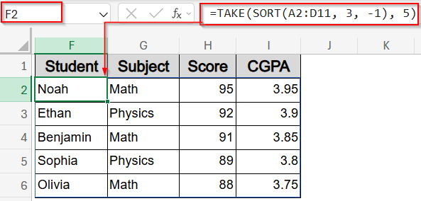
This sorts the dataset by Score (column C) in descending order and returns only the top 5 rows.
Break Ties with RANK and COUNTIF Functions for Unique Rankings
By default, Excel’s RANK function assigns the same rank to duplicate values, which can leave gaps in your ranking. To solve this, you can combine RANK with COUNTIF functions to ensure each entry gets a unique position, even when scores are tied. In our dataset, if two students like Olivia and Sophia had the same score, this method would place one right after the other without repeating the same rank. It’s especially useful when ranking needs to be sequential without skips.
Let’s get started with our modified dataset.
Steps:
➤ In E2, type this formula:
=RANK(C2, $C$2:$C$11, 0) + COUNTIF($C$2:C2, C2) – 1
Here, RANK function assigns the base position, while COUNTIF function counts how many times the same score appeared above, creating unique ranks.
➤ Press Enter.
➤ Drag it down to E11 using the AutoFill handle.
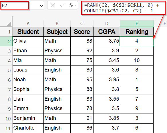
This formula ensures that if two students have the same score, the second one appears ranked just after the first.
Use INDEX and MATCH Functions to Retrieve Students by Rank
To display full student details based on their rank like who scored 1st, 2nd, or 3rd, you can combine INDEX and MATCH functions. This method looks up the student’s name by matching the rank number. Using a helper column with ranks makes it easier to pull records dynamically. For example, enter the rank in the formula to return the student who holds that position, making it perfect for reports or dashboards where you need to show top performers in order.
Steps:
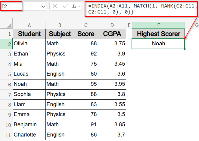
➤ In F2, enter this formula to get the highest scorer:
=INDEX(A2:A11, MATCH(1, RANK(C2:C11, C2:C11, 0), 0))
Here, you can adjust the ranges according to your dataset and also display 2nd, 3rd or other ranks by changing 1 from the formula with the rank number you need.
➤ Alternatively, for a better structure, use helper rank in column E by entering this formula:
=RANK(C2, $C$2:$C$11, 0)

➤ Then, in F2 cell type this formula to return student with Rank 1:
=INDEX(A2:A11, MATCH(1, E2:E11, 0))
➤ Press Enter.
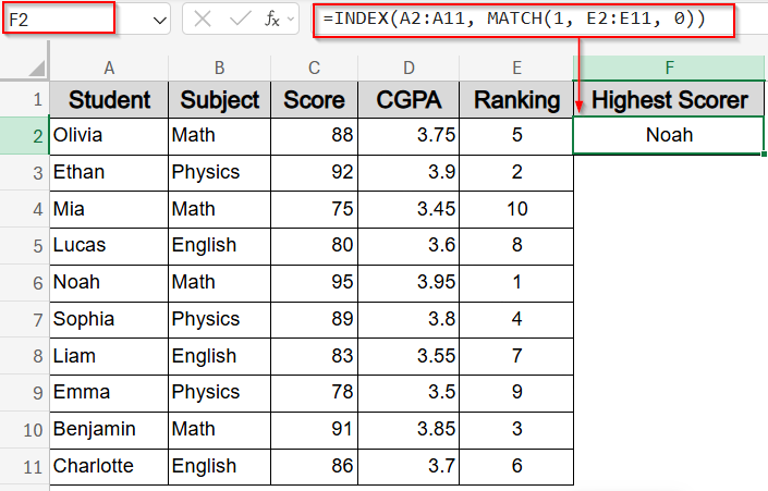
Now you have your highest performer Noah displayed alongside the helper column E.
Use VBA to Auto-Sort and Rank When the Sheet Activates
If you want Excel to automatically sort your data by Score and assign ranks every time you open or activate the worksheet, VBA can do this for you. By adding a simple macro to the sheet’s code module, the data will be sorted in descending order by Score, and ranks will be inserted in column E without any manual effort. This is a great option for automating repetitive sorting and ranking tasks, especially with frequently updated datasets.
Steps:
➤ Open your Excel workbook.
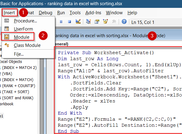
➤ Press Alt + F11 to open VBA Editor, then paste this code into the sheet module using Insert tab >> Module:
Private Sub Worksheet_Activate()
Dim last_row As Long
last_row = Cells(Rows.Count, 1).End(xlUp).Row
Range("A1:D" & last_row).AutoFilter
With ActiveWorkbook.Worksheets("Sheet1").AutoFilter.Sort
    .SortFields.Clear
    .SortFields.Add Key:=Range("C2"), SortOn:=xlSortOnValues, _
    Order:=xlDescending, DataOption:=xlSortNormal
    .Header = xlYes
    .Apply
End With
Range("E2").Formula = "=RANK(C2,C:C,0)"
Range("E2").AutoFill Destination:=Range("E2:E" & last_row)
End Sub
Here, you can change Sheet1 to your original sheet name and change E2 to any output cell you want.
➤ Now press F5 key to run the macro.
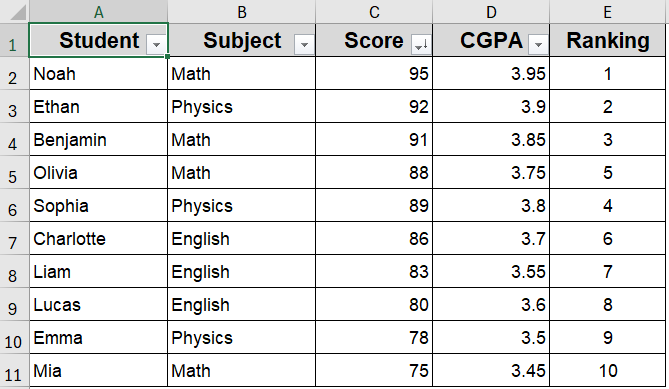
Now, whenever the sheet is activated, Excel will auto-sort by Score and assign ranks in column E.
Frequently Asked Questions
Can I rank without sorting my original data?
Yes, you can assign accurate ranks without changing your original data order. Functions like RANK combined with COUNTIF allow you to calculate ranks based on values directly, keeping the dataset intact and unsorted.
Can I extract the top-ranked student dynamically?
Yes. By using INDEX and MATCH functions alongside a helper column that contains ranks, you can dynamically retrieve full details of the top-ranked student or any rank position without manually searching or sorting your data.
Does RANK automatically break ties?
No, RANK function assigns the same rank to identical values, which results in tied positions. To differentiate tied ranks, you can combine RANK with COUNTIF function to create unique, sequential ranks that avoid skipping numbers after ties.
Do these methods work in older Excel versions?
Most methods except SORT and TAKE functions are compatible with older Excel versions like Excel 2016 and 2013. For the best dynamic functionality, including new array formulas, upgrading to Excel 365 or Excel 2019 and later is recommended.
Wrapping Up
In this tutorial, we learned multiple effective methods to rank data in Excel with sorting, ranging from simple formulas like RANK and COUNTIF to more advanced techniques involving functions like SORT, TAKE, INDEX, MATCH, and even VBA automation. These approaches help you organize and analyze your data clearly, whether you need quick rankings, dynamic top lists, or automated sorting. Feel free to download the practice file and share your feedback.