When analyzing data in Excel, it’s often needed to exclude specific entries to get accurate totals. Whether you’re working with product sales, customer records, or performance metrics, there are times when you want to leave out certain items from your calculations. That might mean excluding a particular product, ignoring rows with missing information, or skipping over a specific category that doesn’t apply to your analysis.
In this article, we’ll learn how to use the SUMIF and SUMIFS function with the “not equal to” (<>) operator to leave out specific values from your totals. These techniques will help you sum only the data you care about whether you’re avoiding blank cells, filtering partial matches, or subtracting specific groups, so your summaries stay accurate and meaningful.
Steps to use SUMIF not equal in Excel:
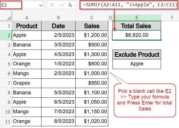
➤ Select a blank cell to display the result (e.g., E2).
➤ Enter the following formula:
=SUMIF(A2:A11, “<>Apple”, C2:C11)
This formula sums all values in the Sales column (C2:C11) where the Product column (A2:A11) is not equal to “Apple“.
➤ Press Enter.
Exclude an Exact Match Using SUMIF Function
One of the most direct ways to filter out specific entries while calculating totals is by using the <> (not equal to) operator with the SUMIF function. This approach is especially useful when you need to exclude a single product from your sales total like summing everything except “Apple“. It’s great for comparative analysis or cleaning reports without deleting rows.
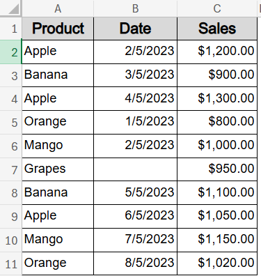
We’ll use a sample dataset containing 10 rows of fruit sales, including product names, sale dates, and amounts. It also includes duplicates and a blank date to demonstrate how to use SUMIF function with <> (not equal) conditions.
Steps:
➤ Select a blank cell to display the result (e.g., E2).
➤ Enter the following formula:
=SUMIF(A2:A11, “<>Apple”, C2:C11)
This formula sums all values in the Sales column (C2:C11) where the Product column (A2:A11) is not equal to “Apple“.
➤ Press Enter.
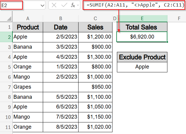
Now Excel will return the total sales from all fruits except “Apple“, giving you a filtered sum without altering your original data.
Dynamically Exclude a Value Using a Cell Reference with SUMIF Function
When working with the SUMIF function, hardcoding the value to exclude can limit flexibility. Instead, you can use a cell reference to make the exclusion dynamic. This means you can change the value to exclude anytime without editing the formula itself. This approach is very useful for interactive reports or dashboards where you want to filter sales totals based on a variable product name such as Apple by typing it in a reference cell.
Steps:
➤ Select a blank cell where you want the total sales result to appear (for example, E2).
➤ In cell E5, type the product name you want to exclude (e.g., Apple).
➤ Enter the following formula in E2:
=SUMIF(A2:A11, “<>” & E5, C2:C11)
This formula sums all sales values in the range C2:C11 where the corresponding product in A2:A11 is not equal to the value typed in cell E5. The <> operator means “not equal to,” and the ampersand & concatenates it with the content of E5, making the condition dynamic.
➤ Press Enter.
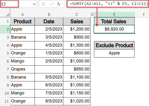
Now, Excel will calculate the total sales excluding the product specified in E5 and the result will update automatically if the value is changed in the same cell.
Apply Multiple Not Equal Conditions with SUMIFS Function
Sometimes, you need to exclude more than one specific value when summing data. The SUMIFS function allows you to apply multiple criteria at once including multiple “not equal to” (<>) conditions. This is perfect when you want to filter out, for example, both a certain product and a particular date from your total sales. Let’s apply this to a dataset where you want to exclude sales of “Apple” and exclude sales on “04/05/2023”.
Steps:
➤ Select a blank cell to display the result (e.g., E2).
➤ Enter this formula:
=SUMIFS(C2:C11, A2:A11, “<>Apple”, B2:B11, “<>4/5/2023”)
This formula sums the values in the range C2:C11 only if the corresponding Product in A2:A11 is not equal to “Apple” and the Date in B2:B11 is not equal to 4/5/2023.
➤ Press Enter.
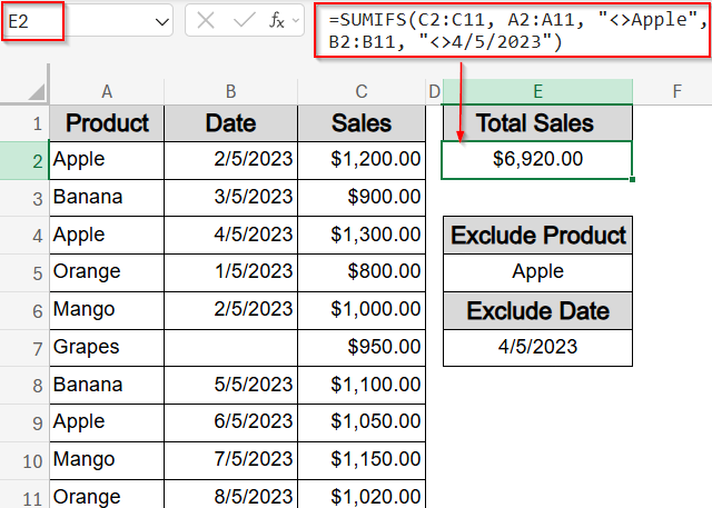
This method is highly effective for complex filtering scenarios, where you want to sum only the data that meets multiple exclusion criteria.
Use Wildcards to Skip Partial Text Matches with SUMIFS Function
If you want to exclude all products that contain certain text anywhere in their name like excluding all fruits that contain the letters “an” (which would exclude “Banana” and “Mango”), this technique is for you. You can do this by combining the “not equal to” (<>) operator with wildcards (*) in your SUMIFS formula. This approach is great for filtering sales based on partial text matches without needing to manually adjust your data.
Steps:
➤ Select a blank cell to show the total (for example, E2).
➤ Enter this formula:
=SUMIFS(C2:C11, A2:A11, “<>*an*”)
This formula sums the sales in C2:C11 only for products in A2:A11 that do not contain the text “an” anywhere in the product name.
➤ Press Enter.
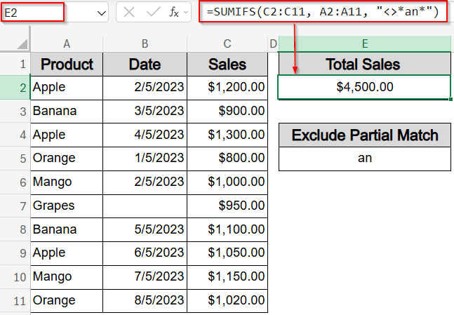
Now Excel will return the total sales excluding all fruits with “an” anywhere in their name such as entries for Banana and Mango in the dataset.
Filter Out Blank or Empty Cells Using SUMIFS Function
When working with real-world data, some rows might have missing or blank entries in important columns like missing dates or products. To ensure your sum only includes complete data, you can use the <> operator with an empty string “” to exclude blank cells. For example, if you want to sum sales only for rows where the Date column is not blank, this method works perfectly.
Steps:
➤ Select a blank cell to display the total (e.g., E2).
➤ Enter the following formula:
=SUMIFS(C2:C11, B2:B11, “<>”)
This formula sums all sales in C2:C11 where the corresponding Date in B2:B11 is not blank. The condition “<>” means “not equal to an empty string,” so any rows with a blank Date will be excluded.
➤ Press Enter.
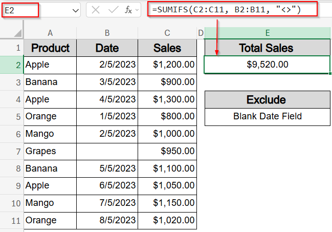
Now Excel will return the total sales amount excluding any rows where the Date field is empty. This is especially useful for ignoring incomplete or missing data in your calculations.
Subtract Multiple Items with SUMIF/SUMIFS Function
Excel’s SUMIF function doesn’t directly allow excluding multiple items with multiple “not equal to” (<>) conditions in one formula. However, you can work around this by calculating the total sum first, then subtracting the sums of the items you want to exclude. For example, to sum sales excluding both “Banana” and “Mango,” you can use this subtraction method. This method is a simple and effective way to exclude multiple products when SUMIF or SUMIFS function don’t natively support multiple “not equal” conditions.
Steps:
➤ Select a blank cell to show the result (e.g., E2).
➤ Type this formula:
=SUM(C2:C11) – SUM(SUMIFS(C2:C11, A2:A11, {“Banana”,”Mango”}))
Here, this formula first calculates the total sales in C2:C11. Then it subtracts the combined sales of “Banana” and “Mango” by summing those specifically with SUMIFS function and an array of items to exclude.
➤ Press Enter.
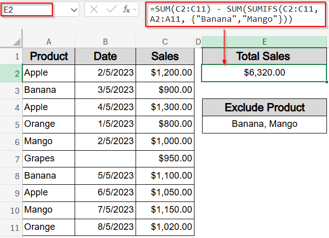
Excel will return the total sales excluding all sales for “Banana” and “Mango”.
Frequently Asked Questions
Can SUMIF function exclude multiple values directly?
No, SUMIF function cannot exclude multiple values at once. You can either use multiple formulas or subtract sums of excluded values using SUMIFS function with arrays, as shown in method 6 for excluding multiple items.
How do wildcards work with SUMIF not equal?
Wildcards like asterisk signs * allow partial text matching. Using <>*text* in SUMIF or SUMIFS functions excludes any entries containing “text” anywhere in the cell, enabling flexible filtering based on partial matches.
Can I use cell references for dynamic exclusions?
Yes. Using a cell reference with the <> operator lets you change the excluded value without editing the formula, making your spreadsheet more flexible and easier to update for different filter criteria.
How do I exclude blank cells in SUMIF or SUMIFS?
Use the condition “<>” to exclude blank cells. This tells Excel to sum only rows where the specified column is not empty, helping you avoid including incomplete or missing data in your calculations.
Wrapping Up
In this tutorial, we explored how to use the SUMIF and SUMIFS functions to exclude values with the “not equal to” operator (<>). We learned multiple practical methods from excluding exact matches and partial text matches with wildcards, to dynamic exclusion with cell references and handling multiple criteria. Feel free to download the practice file and share your feedback.