When working with large datasets in Excel, you may often need to sum values based on more than one condition. The SUMIFS function is designed for exactly this purpose. With the SUMIFS function, you can apply multiple criteria across both columns and rows to extract meaningful insights, especially when your data spans across categories, time periods, or filtered dimensions.
In this article, we’ll walk through the most effective ways to use SUMIFS function with multiple criteria along both columns and rows. We’ll learn how to sum data based on specific categories, dates, non-blank cells, value ranges, and even partial text using wildcards. These methods are ideal for financial analysis, sales tracking, or any task involving multi-dimensional filtering. Let’s get started.
Steps to SUMIFS with multiple criteria in columns and rows in Excel:
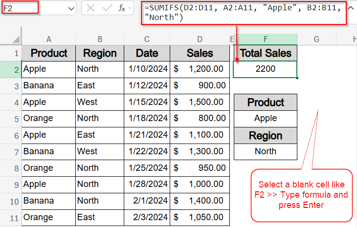
➤ Select a blank cell where you want to return the result (e.g., F2).
➤ Enter the following formula:
=SUMIFS(D2:D11, A2:A11, “Apple”, B2:B11, “North”)
Here, D2:D11 is the numeric range, A2:A11 contains the product names, and B2:B11contains the region headers.
➤ Press Enter.
Use SUMIFS Function with Multiple Criteria in a Vertical Dataset
The SUMIFS function allows you to add up values based on multiple conditions. When your dataset is structured in vertical records with each row representing a complete entry, you can apply criteria across different columns. For example, if you want to know the total sales for “Apple” in the “North” region, you can filter by both the Product and Region columns simultaneously.
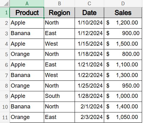
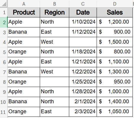
We’ll use a sample dataset containing product names, regions, dates, and sales figures to demonstrate how SUMIFS function works with multiple criteria across rows and columns.
Steps:
➤ Select a blank cell where you want to return the result (e.g., F2).
➤ Enter the following formula:
=SUMIFS(D2:D11, A2:A11, “Apple”, B2:B11, “North”)
Here, D2:D11 is the numeric range, A2:A11 contains the product names, and B2:B11contains the region headers.
➤ Press Enter.
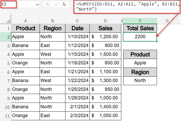
Now Excel will return the value where the product is “Apple” and the region is “North“.
Apply SUMIFS function with Comparison Operators and Dynamic Cell References
This method helps you sum values based on criteria that change dynamically. Instead of hardcoding numbers into your formula, you can use cell references along with comparison operators. Our goal here is to sum only those values that meet multiple flexible conditions like matching a region like North and falling below a certain numeric threshold such as 1100.
Steps:
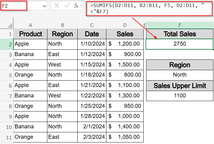
➤ Select an empty cell where you want to see the result (e.g., F2).
➤ Enter the following formula:
=SUMIFS(D2:D11, B2:B11, F5, D2:D11, “<“&F7)
Here, D2:D11 is the range to sum, B2:B11 checks for a specific region stored in D5, and the formula adds an upper limit by referencing D7.
➤ Press Enter.
➤ You can now change the values in F5 and F7 anytime to update the result automatically.
This method is especially helpful when you want your formula to respond to different filter values without rewriting it every time.
Insert SUMIFS Function with Non-Blank Cell Criteria in Columns and Rows
When working with real-world data, some entries may be incomplete. In such cases, it’s helpful to sum values only when certain supporting columns like Date or Region that aren’t blank. Our goal here is to include only complete rows by excluding those with missing values in either column when finding out Total Sales.
Let’s begin with our modified dataset.
Steps:
➤ Select an empty cell where you want to display the result (e.g., F2).
➤ Enter the following formula:
=SUMIFS(D2:D11, B2:B11, “<>”, C2:C11, “<>”)
Here, D2:D11 is the range to sum, B2:B11 filters out rows where the Region is blank, and C2:C11 filters out missing Date.
➤ Press Enter.
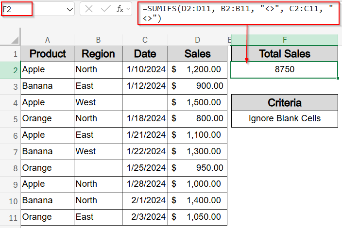
Now the result will update automatically whenever blank cells are added or removed from our dataset. This method is ideal for ensuring your totals reflect only valid and complete data entries.
SUMIFS Function with Multiple Row Criteria Including OR Logic
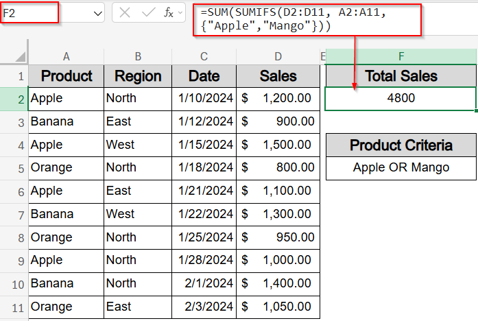
Sometimes, you may need to sum values based on more than one matching item, such as totals for “Apple” or “Mango“. The SUMIFS function doesn’t natively support OR logic within a single call, but you can wrap it inside a SUM function along with an array to handle multiple criteria. Our goal here is to sum values across multiple specified months using a single formula.
Steps:
➤ Click on an empty cell where you want the total to appear (e.g., F2).
➤ Type the formula:
=SUM(SUMIFS(D2:D11, A2:A11, {“Apple”,”Mango”}))
This formula adds up the values in D2:D11 where the corresponding cell in A2:A11 matches either “Apple” or “Mango“.
➤ Press Enter to calculate the result.
This technique is especially useful when you’re aggregating values across custom groupings like quarterly, seasonal, or bi-monthly periods.
Combine SUMIFS Function with Wildcards for Partial Matching
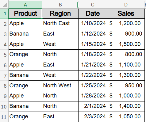
In many datasets, values may begin with a common prefix like a customer ID or region tag, but vary afterward. In such cases, you can use wildcards with SUMIFS to match partial entries. Our goal in this method is to sum only the rows where a specific column starts with a common prefix, such as “North“. We will use the following modified dataset:
Steps:
➤ Select an empty cell where you want the result to appear (e.g., F2).
➤ Enter the following formula:
=SUMIFS(D2:D11, B2:B11, “North*”)
This formula checks the values in B2:B11 for entries that begin with “North” and sums the corresponding values in D2:D11.
➤ Press Enter to get the total.
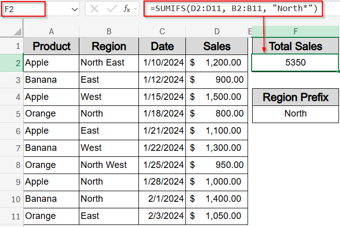
The asterisk (*) works as a wildcard to match any number of characters after “North“. This method is ideal for partial code matches, prefix-based categories, or filtering similar labels efficiently.
Use SUMIFS Function with Multiple Criteria Along Columns and a Date Range
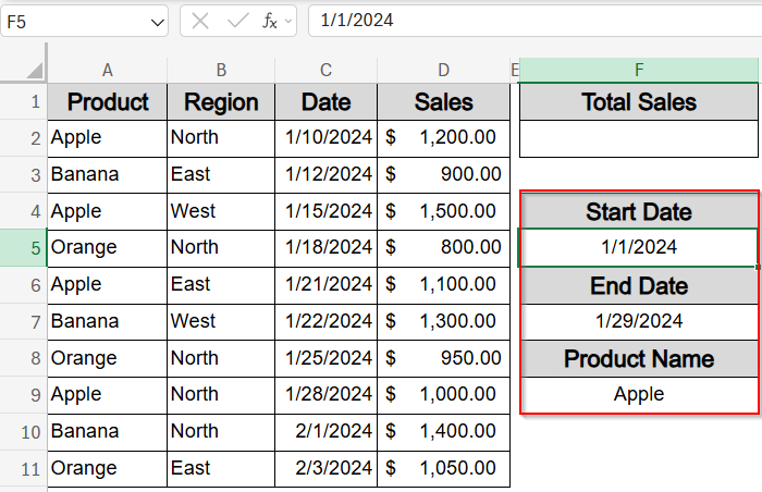
When analyzing time-based data like sales, attendance, or transactions, it’s common to filter by both date ranges and categories. This method uses SUMIFS function to sum values that meet multiple conditions across columns such as matching a product name like Apple and falling within a specific time window such as 1st January, 2024 to 29th January, 2024.
Steps:
➤ Type your Start Date, End Date and Product Name in cells F5, F7 and F9 respectively for setting up the criteria.
➤ Select a blank cell where you want the result to appear (e.g., F2).
➤ Enter the following formula:
=SUMIFS(D2:D11, C2:C11, “>=”&F5, C2:C11, “<=”&F7, A2:A11, F9)
Here, D2:D11 is the range to sum, C2:C11 contains dates, and A2:A11 holds categories or names. The cells F5 and F7 store the start and end dates, while F9 contains the specific item to match.
➤ Press Enter to get the total sum within the set criteria.
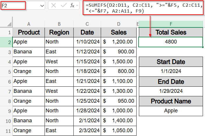
This method is perfect for generating monthly reports, tracking sales by period, or filtering values by date and category by using a single dynamic formula.
Apply SUMIFS Function with Multiple Criteria and a Numeric Range
This method is ideal when you want to sum only the numbers that fall within a specific numeric range such as prices between 1100 and 1500 or test scores within a grading band. You can apply multiple numeric criteria within the same column to filter your data precisely. Let’s get started.
Steps:
➤ Click on an empty cell where you want the result to appear (e.g., F2).
➤ Enter the following formula:
=SUMIFS(D2:D11, D2:D11, “>1100”, D2:D11, “<1500”)
Here, D2:D11 is both the range to sum and the range being filtered. The formula adds values greater than 1100 and less than 1500.
➤ Press Enter to calculate the result.
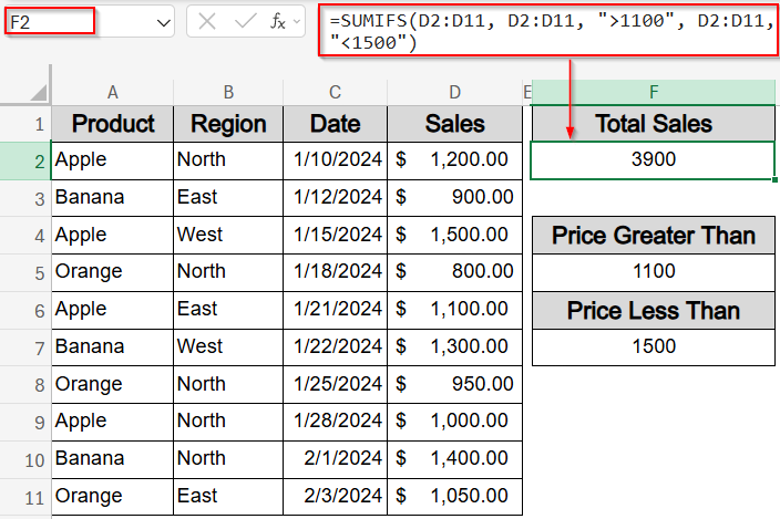
This approach is perfect for quickly summing mid-range values such as moderate sales amounts, specific score brackets, or filtered inventory quantities.
Frequently Asked Questions
What’s the difference between SUMIF and SUMIFS in Excel?
The SUMIF function allows you to apply a single condition to a dataset, while SUMIFS function lets you apply multiple criteria across different columns, making it ideal for complex filtering and multi-dimensional data analysis.
Can I use OR logic with SUMIFS in Excel?
While SUMIFS function is designed for AND logic, you can simulate OR logic by nesting multiple SUMIFS functions inside a SUM formula and using array constants like {“Apple”,”Mango”} for multi-item summing.
How do I use wildcards with SUMIFS?
You can use asterisk sign (*) to represent any number of characters or ? for a single character in your criteria. This helps you match partial entries such as names, codes, or product IDs.
Why is SUMIFS not working with dates?
SUMIFS function may fail if your date values are stored as text or mismatched in format. Ensure all date cells are properly formatted, and use logical operators like “>=”&A1 to apply conditions.
Can SUMIFS be used across different sheets?
Yes, you can use the SUMIFS function across sheets by referencing ranges like ‘Sheet2’!A2:A10, but ensure all ranges are the same size and the formula syntax is consistent throughout to avoid errors.
Wrapping Up
In this tutorial, we explored how to use the SUMIFS function with multiple criteria across both rows and columns in Excel. Whether you’re matching specific items, filtering by date ranges, using wildcards, or summing within numeric conditions, these methods help you perform powerful multi-dimensional analysis without complex tools. Feel free to download the practice file and share your feedback.