Looking up values based on multiple criteria is a common challenge in Excel because the VLOOKUP function natively supports only a single lookup value. To overcome this, you can use several practical techniques to perform lookups with two lookup values, ensuring accurate results without complex formulas or additional tools.
In this article, you will learn several effective methods to use VLOOKUP with two lookup values by adding a helper column, using the CHOOSE function to create a virtual lookup table, and nesting multiple VLOOKUP functions. Let’s get started.
Steps to use VLOOKUP with two lookup values in Excel:
➤ In F1 and G1 cells, enter column headers such as First Name and Last Name.
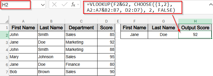
➤ In F2, type the first name you want to look up (e.g., Jane), and in G2, the last name (e.g., Doe).
➤ In H1, type Output Score. Then in H2, enter the formula:
=VLOOKUP(F2&G2, CHOOSE({1,2}, A2:A7&B2:B7, D2:D7), 2, FALSE)
➤ Press Enter.

Helper Column Method for VLOOKUP Function with Two Lookup Values
The simplest way to make VLOOKUP handle two lookup values is by adding a helper column that merges both into one searchable key. This approach is fully compatible with all Excel versions and requires no advanced formulas.
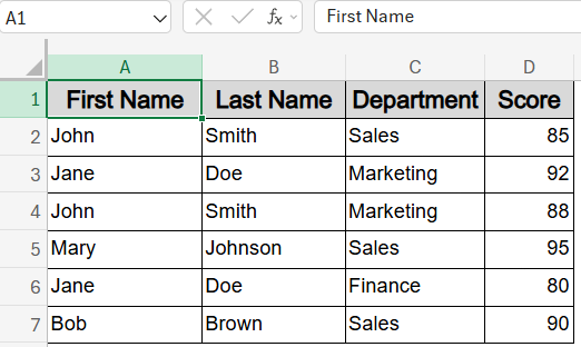
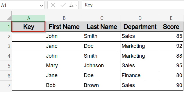
We’ll use a sample dataset containing employee records with four columns: First Name, Last Name, Department, and Score. By combining the first and last names into a single “Key” column, we can return the correct Score using a standard VLOOKUP function. For instance, searching for “JaneDoe” will dynamically return 92 from the Marketing department.
Steps:
➤ Insert the header Key in cell A1 as your helper column.

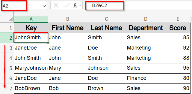
➤ In A2 enter this formula to combine First Name and Last Name such as JohnSmith:
=B2&C2
➤ Press Enter and drag down through A7 using the AutoFill handle.

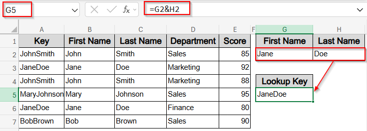
➤ Type your two lookup values manually like Jane and Doe in cell G2 and H2 respectively.
➤ Enter formula in G5 cell:
=G2&H2
This will link G2:H2 to G5 cell so that the Lookup Key is automatically generated by merging names such as JaneDoe.
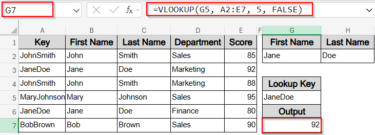
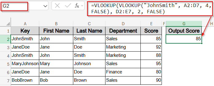
➤ Use this formula in G7 to find the Score:
=VLOOKUP(G5, A2:E7, 5, FALSE)
➤ Hit Enter.
This searches the Key column and returns the corresponding Score from column D which is 92.
Now your dataset cleanly converts two lookup values into one key for VLOOKUP, keeping your worksheet simple and efficient.
Note: Instead of changing your dataset or adding helper columns, this method uses the CHOOSE function to create a virtual table directly inside the formula. It pairs First Name and Last Name with Score using an in-memory array. When you search for Jane and Doe, the combined result JaneDoe correctly returns 92 from the dataset. Steps: ➤ In F1 and G1 cell, enter column headers such as First Name and Last Name. ➤ In H1, type Output Score. Then in H2, enter the formula: =VLOOKUP(F2&G2, CHOOSE({1,2}, A2:A7&B2:B7, D2:D7), 2, FALSE) The formula combines values from A2:A7 and B2:B7 to simulate a lookup key (e.g., JaneDoe) and matches it to the corresponding Score in D2:D7. ➤ Press Enter. Now you have your corresponding output such as 92 matching the lookup criteria like Jane and Doe in your dataset. This method performs a two-step lookup by nesting one VLOOKUP function inside another. Instead of merging the lookup values, the formula first finds the department for the first matching name, such as “JohnSmith“, and then uses that department to retrieve the related Score. For example, the first “JohnSmith” entry is in Sales, so the formula returns a Score of 85. This approach works well when the result depends on the first matching value in a step-by-step lookup. Steps: ➤ Insert the header Key in cell A1 as your helper column. ➤ In A2 enter this formula to combine First Name and Last Name such as JohnSmith: =B2&C2 ➤ Press Enter and drag down through A7 using the AutoFill handle. ➤ Use the following nested formula to look up the Score for “JohnSmith“: =VLOOKUP(VLOOKUP(“JohnSmith”, A2:D7, 4, FALSE), D2:E7, 2, FALSE) ➤ Press Enter. This two-layer logic returns 85, resolving the name to a department and then using that to get the score. While it won’t handle duplicates dynamically (like skipping to a second match), it’s useful when data is structured so that one lookup leads into another in a meaningful sequence. Yes, by using the CHOOSE function inside VLOOKUP, you can create a virtual combined lookup array. This avoids extra columns but requires understanding of array formulas and may be less intuitive for beginners. No, nested VLOOKUPs perform sequential lookups but don’t handle duplicates or return multiple matches. They return the first matching result. For duplicates, formulas like INDEX with SMALL or FILTER (Excel 365/2021) are better suited. The helper column method is simplest and most reliable for older Excel versions. It requires no advanced functions or arrays and works by concatenating lookup values into a single column, making it easy to implement across all Excel versions. In this tutorial, we learned three practical ways to use VLOOKUP with two lookup values effectively. Whether you prefer creating a helper column, using the CHOOSE function for a dynamic virtual table, or nesting VLOOKUPs for sequential lookups, these techniques will improve your data retrieval skills and simplify your Excel workflows. Feel free to download the practice file and share your feedback.
Adjust cell references if your data expands.VLOOKUP with Two Lookup Values Using CHOOSE Function
➤ In F2, type the first name you want to look up (e.g., Jane), and in G2, the last name (e.g., Doe).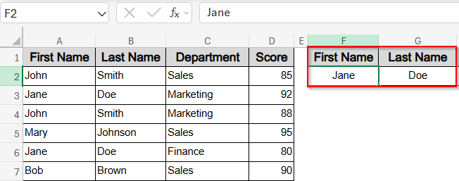
VLOOKUP with Two Lookup Values Using Nested Functions
Frequently Asked Questions
Can I use VLOOKUP to search for two values without adding a helper column?
Will the nested VLOOKUP method handle duplicate lookup values automatically?
Which method is best for older Excel versions?
Wrapping Up