In accounting, the weighted average is often used for inventory calculations. Instead of the normal average, weighted averages sometimes provide a better picture of the data for various statistical analysis. In this article, we will learn to do a weighted average excel pivot table instead of doing it in regular data range.
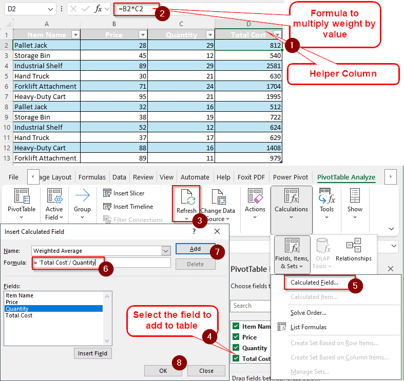
➤ Add a helper column to your source table with the multiplication of weight and values. Use a formula like this to do it: =B2*C2
➤ Go to the pivot table, refresh it, and select the new helper column from the PivotTable Fields panel to add it.
➤ Head to PivotTable Analyze tab and find Fields, Items, & Sets from the Calculations group to add a Calculated Field.
➤Use the formula to divide the helper column with the values. = ‘Total Cost’/ Quantity
➤ Replace ‘Total Cost’ with the helper column and Quantity with the values and hit Add.
It is easy to get confused by many steps. But not to worry, because we have the full procedure explained in this tutorial step-by-step for you. Therefore, read the whole article to understand the process so that you can apply it to your dataset as well.
What is Weighted Average?
In general, average is calculated by dividing the sum of something by the count. For example, if you bought 10 pens for 90 dollars, we could calculate that each pen costs 9 dollars by dividing 90 by 10. This is useful when each pen costs the same, so the average makes sense.
However, if you buy 5 pens for 40 dollars, and 5 more for 50 dollars, you get two averages. The first average for 5 pens is 8 dollars, and the second average is 10 dollars for 5 pens. Those are two regular averages. But when you add up these numbers and divide, you get the weighted average. Now the calculation will be (40+50)/(5+5)=9 dollars.
For bigger calculations, like in accounting, inventory is often calculated using the weighted average method to calculate the price. Doing the calculation in excel is easy, but not so much in a pivot table. Let’s learn how we can do that in a pivot table.
Steps to Calculate Weighted Average in Excel Pivot Table
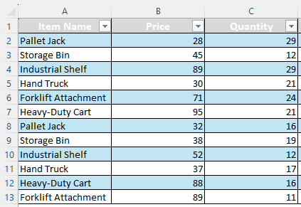
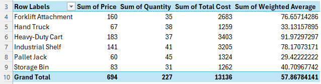
For today’s calculation, we have some items at a warehouse. The items for the warehouse are bought at different prices and in different quantities. We want to calculate the average prices of each item using the weighted average.
Follow the procedure below to do the calculation:
Step 1: Add a Helper Column
First, we need to add a helper column that will multiply the price by the quantity. Then we will create a pivot table to work with it.
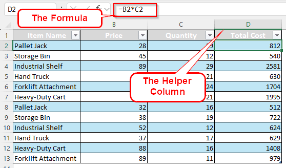
➤ In the D2 cell (As we will use D1 as the heading), write the following formula:
=B2*C2
➤ Upon pressing Enter, excel should automatically add the new column to the table while filling the rest of the cells at the same time.
➤ Rename Column1 to Total Price because that’s what it is.
Step 2: Create the Pivot Table
Now we have to create the pivot table where we will actually calculate the weighted average.
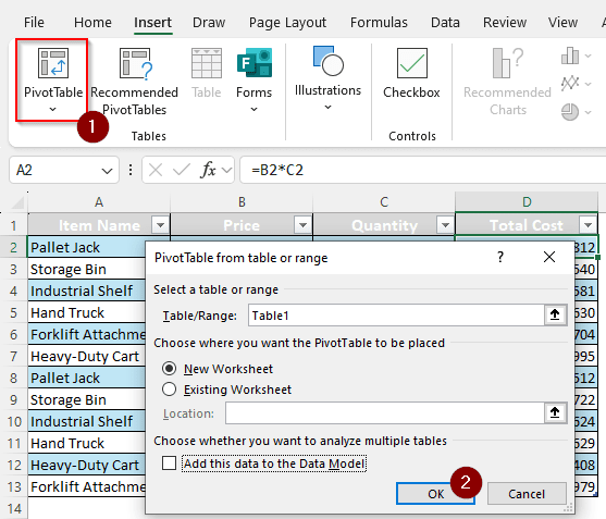
➤ Select any cell of the table and go to the Insert tab to select PivotTable.
➤Press OK in the new window to create the pivot table.
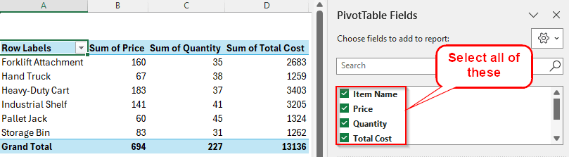
➤ Go to the pivot table and select all of the fields to make the table show up.
Step 3: Add a Calculated Field
For the final step, we will use a calculated field to complete the job. The helper column will be divided by the quantity, and the weighted average will come as output.
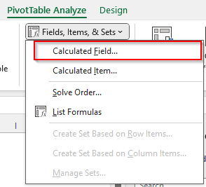
➤ Click on a cell of the pivot table. Then go to the PivotTable Analyze tab.
➤ In the Calculations section, open the drop-down menu of Fields, Items, & Sets and click on Calculated Field.
➤ In the new window, change the Name to Weighted Average, and write this formula:
='Total Cost'/ Quantity
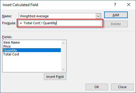
➤ Press Add and OK.
Frequently Asked Questions
How do I do a weighted average in Excel?
Write the formula like this:
=SUM(B2:B13 * C2:C13)/ SUM(C2:C13)
Replace B2:B13 with the range of the weight and C2:C13 with the range of the value.
How to calculate weighted average in sheet?
Use this formula:
=SUMPRODUCT(A2:A4, B2:B4) / SUM(B2:B4)
Replace A2:A4 with the range of weights and B2:B4 with the range of values.
How to use sumproduct?
SUMPRODUCT is basically the same as multiplying two sums in a formula. The function is written like this:
=SUMPRODUCT(A1:A2,B1:B2)
Here, A1:A2 and B1:B2 cells are added first, then multiplied with each other.
How do you calculate the general average?
Just add the values and divide by the count. The formula in Excel can be written like this:
=SUM(A1:A10)/10
Here, the values in A1:A10 are summed up, then divided by 10 as there are ten cells in the range.
How to find weighted mean in Excel?
Weighted mean and weighted average are the same. The methods mentioned in this article can be used to calculate both.
Wrapping Up
In this article, we learned how to calculate weighted average excel pivot table. The Excel file used in this tutorial is available for you to download. We always appreciate feedback, so comment down on how you found this tutorial helpful for your job. We will meet again in another tutorial.