Pivot tables are very useful for data analysis in Excel. In order to ease our analysis, we can use different layouts in a pivot table. In this article, we will learn how to change pivot table layout in Excel in detail.
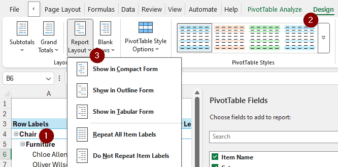
➤ Click on any row of your pivot table.
➤ Go to the Design
➤ From the Layout section, open the Report Layout dropdown menu, and select your desired layout.
Those are the basic layouts you can use to customize your pivot table with. However, there are a lot of other customization options that you can use for your convenience. Therefore, keep reading the whole article to know the methods you can use to change pivot table layout according to your choice.
Changing the Basic Layout
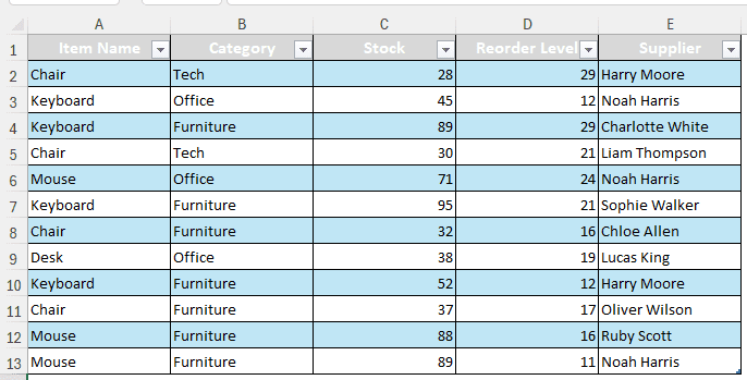
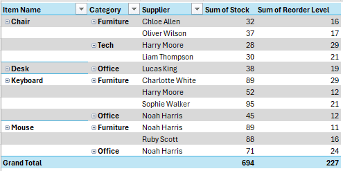
In this tutorial, we have a dataset of some product inventory. We have the Stock and Reorder levels, and because of the pivot table, we can inspect the data better. We are going to change the layout of this pivot table.
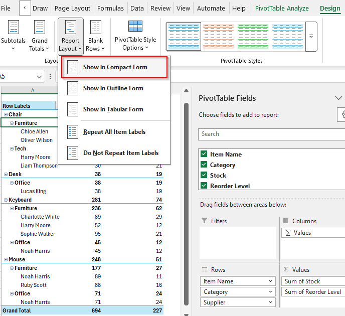
➤ Select one of the cells of the table for the Analyze and Design tabs to show up.
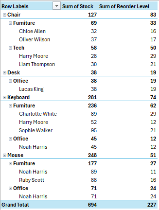
➤ Go to Design > Report Layout > Show in Compact Form. Nothing will change because this is the default layout.
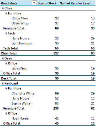
➤ Select Show in Outline Form. Now the columns are expanded.
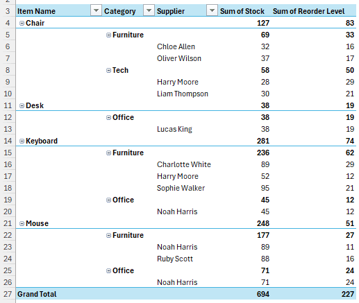
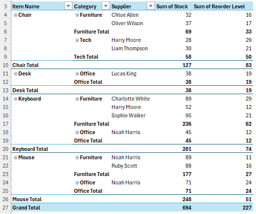
➤ Select Show in Tabular Form. Now individual sums are visible in a different way.
Formatting a Pivot Table Further
Those were the basic layouts of a pivot table. However, Excel allows us to customize more. We will learn more about changing the pivot table layout in this section:
Changing the Totals Layout
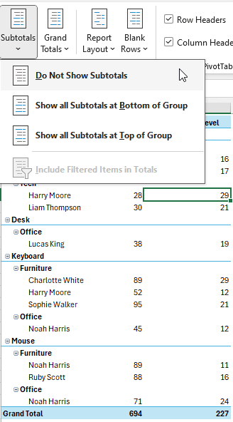
➤ From the Design tab, select Subtotals > Do Not Show Subtotals. Now the subtotals of each category are not shown:
➤ Changing to Show all Subtotals at Bottom of Group will do as the option suggests. The subtotals will be shown under each group.
➤ Change to Show all Subtotals at Top of Group to see the subtotals at the top.
➤ Play with the Grand Totals option to make the grand total visible when needed.
![]()
Customizing the Rows
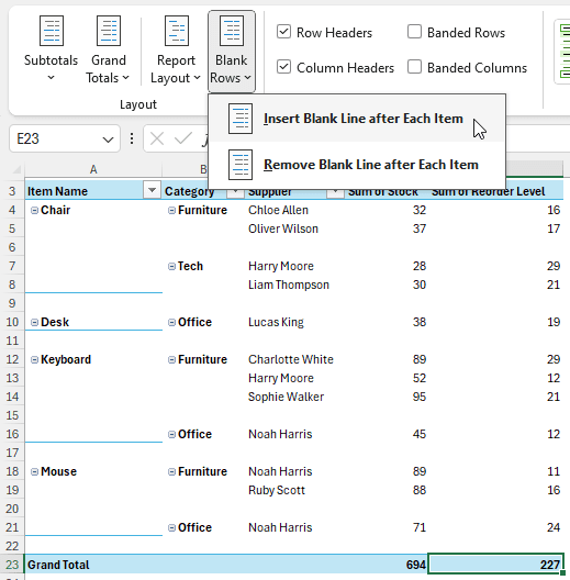
➤ Go to Blank Rows > Insert Blank Line after Each Item to add blank rows for better visibility.
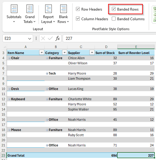
➤ From PivotTable Style Options, check the Banded Rows box to identify the rows better.
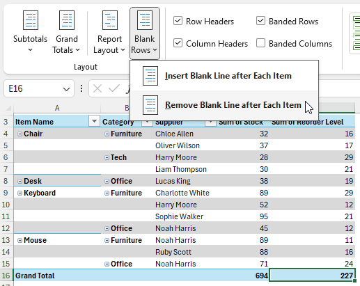
➤ Now you can remove the blank rows by selecting Remove Blank Line after Each Item and keep the banded rows for compactness.
Using VBA Script to Change Layout
We are going to use some advanced tactics to change the layout of the pivot table. Using some VBA code, we can change the pivot table layout without touching the UI. Here is how we do it:
➤ Press Alt+F11 to open the VBA IDE.
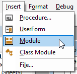
➤ Go to Insert > Module.
➤ Write this code in the code editor:
Sub ChangePivotTableLayout(layoutType As String)
    Dim pt As PivotTable
    Set pt = ThisWorkbook.Sheets("InventoryPivot").PivotTables("PivotTable1")
    Select Case layoutType
        Case "Tabular"
            pt.RowAxisLayout xlTabularRow
        Case "Outline"
            pt.RowAxisLayout xlOutlineRow
        Case "Compact"
            pt.RowAxisLayout xlCompactRow
        Case Else
            MsgBox "Invalid layout type. Please use 'Tabular', 'Outline', or 'Compact'."
    End Select
End Sub
Sub ChangeToTabular()
    ChangePivotTableLayout "Tabular"
End Sub
Sub ChangeToOutline()
    ChangePivotTableLayout "Outline"
End Sub
Sub ChangeToCompact()
    ChangePivotTableLayout "Compact"
End Sub
➤ Replace “InventoryPivot” with your pivot table sheet, and “PivotTable1” with your pivot table name.
➤ Press F5 and select which layout you want to see your table in.
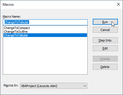
➤ Hit Run, and you will see that the pivot table layout has been changed.
Frequently Asked Questions
How do I change the style of a PivotTable in Excel?
When you have selected a row for your pivot table, go to the Design tab. In the PivotTable Styles section, you will see a lot of predetermined styles. Select one of them, or use the dropdown menu and create your own style.
How do I change the default PivotTable settings in Excel?
From the File menu, go to Options. From the new window, select Data from the left panel. On the right, you will see an option called “Make changes to the default layout of PivotTables”. From there, click on “Edit Default Layout”. You can customize the default pivot table settings from there.
How to change PivotTable layout to classic?
Select any cell of your pivot table. Right-click on that and select PivotTable Options. A new dialog will open. Go to the Display tab, and check “Classic PivotTable Layout (enables dragging of fields in the grid)”.
How do I reset my PivotTable?
When you have a cell of the pivot table selected, go to the PivotTable Analyze tab. From the Actions section, go to Clear > Clear All. This will reset your pivot table.
How to sort a PivotTable?
Right-click on one of the cells in a pivot table and select Sort. From there, you can sort from smallest to largest and vice versa. You can even select custom sorting options if you want.
Wrapping Up
In this article, we have learned all about how to change pivot table layout in Excel. You can download the exercise workbook to work on enhancing your skills. Leave a comment with your suggestions, and we will see you in another tutorial.