
Pivot Tables are used for various types of data analysis. While columns are used for major sections of a dataset, sometimes we need to modify the table to show the rows in columns. In this article, we will learn how to put pivot table row labels in separate columns in Excel.
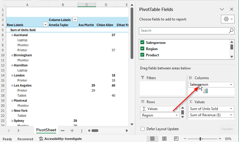
➤ Select a cell of your pivot table so that the “PivotTable Fields” panel on the right shows up.
➤ On the bottom right, notice that there are some areas called Filters, Columns, Rows, and Values.
➤ Take the row labels you want to show as columns and drag them to the column area.
If the key takeaway was too short for you, we have the step-by-step guide written below for your convenience. Consider reading the whole article to learn more about pivot tables and putting pivot table values in column not row. Without wasting any more time, let’s begin.
Putting Row Labels in Separate Columns in Excel
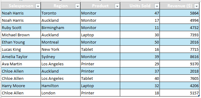
Here, we have some sales performance data. The table contains the names of the salespersons, the regions where they sold the products, the types of products, the units, and the revenue. Those are the column headings, but we want to check each salesperson’s performance, which is shown in rows.
Step 1: Create the Table
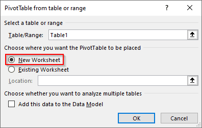
➤ Select the dataset, and go to Insert > PivotTable
➤ Select a new worksheet and hit OK
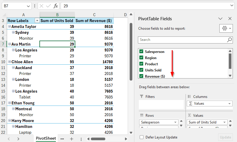
➤ After selecting the required fields, the pivot table looks something like this:
Step 2: Transform Rows to Columns
➤ The salesperson’s names are shown in the Row Labels column, and the places they worked are in a tree view.
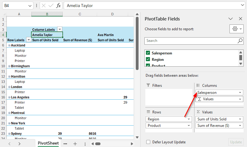
➤ From the bottom right, we drag the Salesperson field from Rows to Columns.
Rearranging the Table
Instead of messing with the pivot table, we can create a new table in Excel by transferring the rows to the columns and vice versa. Here is how to do that:
Step 1: Transpose the Rows and Columns
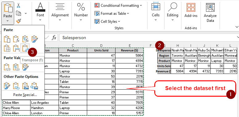
➤ Select the dataset, and click Ctrl+C.
➤ Go to another cell with enough blank cells on the right and the bottom to put the new table in.
➤ From the Paste menu, select
Note:
You can use a formula to do the transposition as well. In the new cell, write this:
=TRANSPOSE(A1:E13)
Replace A1:E13 with the data range of your table.
Step 2: Create a Pivot Table
➤ Select the transposed dataset and press Ctrl+T to create a new table.
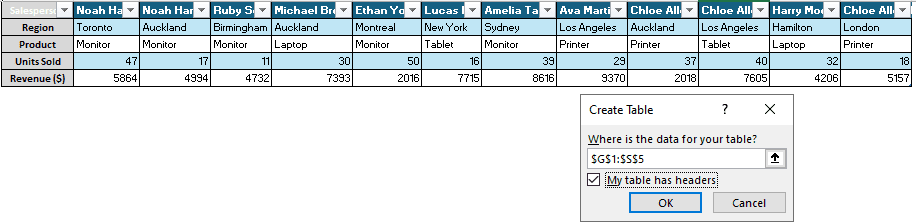
➤ Now, go to Insert > PivotTable and create a new pivot table.
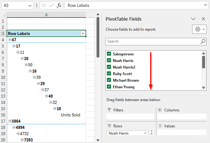
➤ From the new pivot table, we select all the columns to let them show up.
Step 3: Format the Pivot Table
This sheet looks a lot messed up. That’s because Excel shows everything in compact view by default, and the data is not properly formatted because of that.
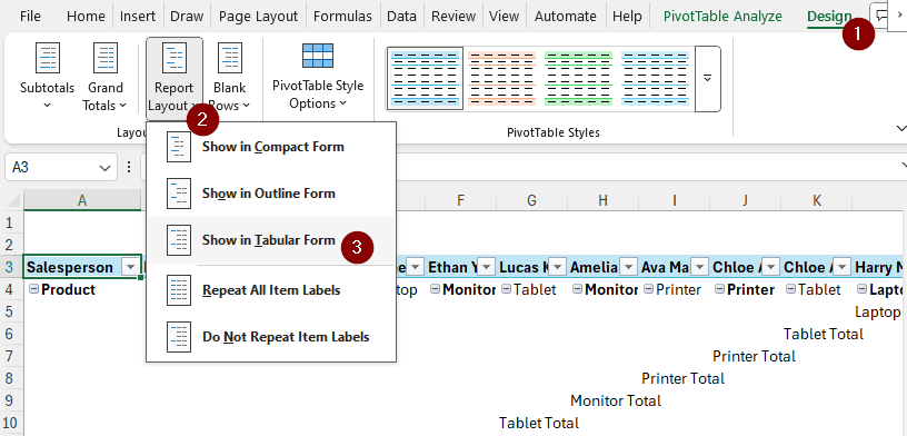
➤ Go to Design tab and select Report Layout > Show in Tabular Form. Now the pivot table is properly shown with rows and columns.
Downloadable Resources
Get our practice workbook or necessary files that we have worked with to prepare this article.
Transfer Pivot Table Row Labels in Separate Columns.xlsx
Frequently Asked Questions
How to manually sort PivotTable columns?
Click on the small arrow on the heading of a column and select the fields you want to sort. In order to sort those in ascending or descending order, click on Sort A to Z or Sort Z to A.
How do I separate data from rows to columns?
Select your data in Excel. Then go to Data > Data Tools > Text to Columns. From the new wizard, you can convert your data from rows to separate columns.
How to change column labels in pivot table?
Decide which column you want to change the label of. Then click on the heading of the column twice. A new dialog will pop up with the label “Value Field Settings”. From there, you can change the name of the column and hit OK to confirm.
How do I add a row label filter in a pivot table?
Select a cell from the pivot table to bring up the “PivotTable Filters” panel. From there, drag the row label in the Filters box. The data will now be filtered according to the label you selected.
How to resize pivot table field list?
Using the mouse cursor, go to the edge of a pivot table until the cursor turns into a plus (+) sign. Then drag the mouse while holding the left button to resize the fields.
Wrapping Up
From this article, we learned how to transform pivot table row labels in separate columns. The workbook we used for this tutorial has the example included, and you can download and use it for your convenience. If you find any difficulties using the methods in the article, leave a comment, and we will get back to you as soon as possible.