In Microsoft Excel, getpivotdata is an excellent function to look up data from a pivot table. While Excel itself suggests using this function while using pivot tables, it is not dynamic by default. In this article, we will learn how to use getpivotdata dynamic referencing so that we can modify our pivot table without losing the references in the getpivotdata formula.
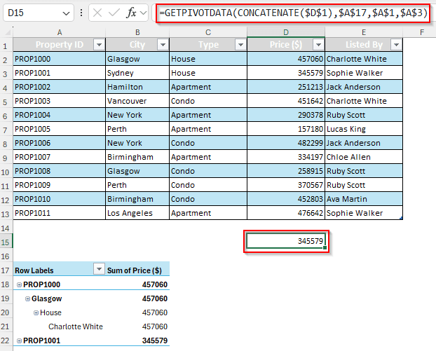
➤ Write the formula in your desired cell:
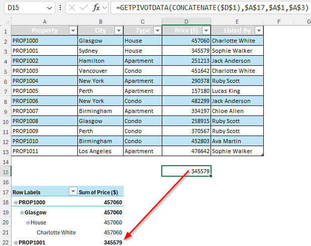
=GETPIVOTDATA(CONCATENATE($D$1),$A$17,$A$1,$A$3)
➤ Replace $D$1 with your data field from the source table, $A$17 with the cell from where the pivot table starts, $A1$1 with the field, and $A$3 with the item.
➤ Press Enter
That takeaway was precise, but also confusing if you are less familiar with the functions and references used in the formula. In this tutorial, we will have the full explanation of the formula, and some more techniques to do the dynamic referencing in getpivotdata function. Therefore, consider reading the whole article to get a good grasp of the formula.
What is GETPIVOTDATA Function in Excel?
GETPIVOTDATA is a function that extracts data from a pivot table. The function syntax is written like this:
=GETPIVOTDATA(data_field, pivot_table, [field1, item1], [field2, item2], …)
Here, the data_field must be a string value, basically a column/row header, from which a datapoint will be extracted. A cell reference is not accepted in this parameter. Next, pivot_table refers to the pivot table itself, however, this parameter refers to the cell where the pivot table starts from. Finally, there could be an array of parameters with fields and items that help narrow down the desired value. The function essentially works as a VLOOKUP alternative for pivot tables.
Using Dynamic Reference in GETPIVOTDATA
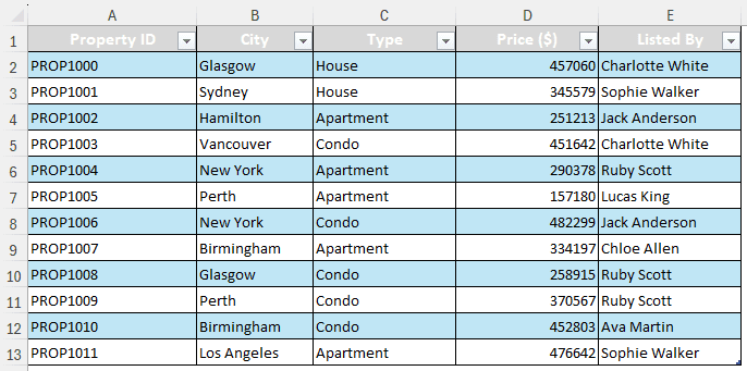
For this tutorial, we are using a sample dataset with some real estate listings. There are property IDs, cities where the properties are located, types of the properties, prices, and the names of the people who have listed them. We are going to use the GETPIVOTDATA function to extract data from the pivot table created from this source data.
Step 1: Using GETPIVOTDATA
➤ On a cell outside of the pivot table, write the equal sign (=), and select a cell inside the pivot table.
➤ Excel will automatically use the GETPIVOTDATA function for referencing the cell from the pivot table.
➤ Upon pressing Enter, the value will be displayed from the pivot table.
➤ However, if we change the pivot formatting, the value will disappear, and it will display an error (#REF) in the cell. For example, we changed the name of the Property ID field to Property, refreshed the table, and added the field back. Here is the result:
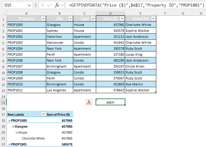
➤ The formula still says, “Property ID” instead of “Property”, so the function cannot refer to the correct cell. We need to use dynamic referencing to solve this issue.
Step 2: Changing Static References to Dynamic References
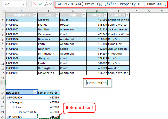
➤ Let’s take a look at the formula Excel has given us.
=GETPIVOTDATA(“Price ($)”,$A$17,”Property ID”,”PROP1001″)
➤ The formula finds the value from the column that’s named Price ($). The pivot table is from $A$17 cell, the field is Property ID, and the item is PROP1001. We would change it to the following:
=GETPIVOTDATA(CONCATENATE($D$1),$A$17,$A$1,$A$3)
For the next parameter, we keep the $A$17 value as it is the pivot table reference, which has not changed. The next parameter is the field, we write $A$1 here as that is the cell of the source column which refers to the Property column (Remember, we changed Property ID to Property in the first step to highlight the issue). Finally, $A$3 is the item, which is basically PROP1001.
For the first parameter, instead of using CONCATENATE($D$1), you can use TEXT($D$1,””), “” & $D$1 & “”. They all convert the source cell to text.
➤ Press Enter
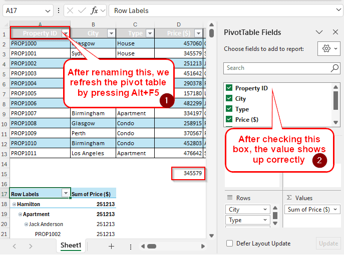
➤ To verify that the function is working properly, we rename the A1 cell to Property ID, refresh the pivot table by pressing Alt + F5 , and add the field to the pivot table.
Frequently Asked Questions
How do I create a dynamic reference in Excel?
Use this function:
=INDIRECT(B2)
Here, Excel returns the reference from the B2 cell, while that cell can refer to another cell.
What is dynamic referencing?
In Excel, dynamic referencing is referring to a cell instead of a static datapoint, allowing the datapoint to be changed whenever required without affecting the reference.
What are dynamic formulas?
Dynamic formulas use an array for the parameters instead of a limited number of values.
Do PivotTables dynamically update?
Pivot tables can be dynamically changed whenever required, but they do not update dynamically. You need to refresh the pivot table to update it.
What is a dynamic table in Excel?
In a dynamic table, the user can add/remove/update values whenever they want without having to change the table structure every time.
Wrapping Up
In this article, we have learned how to use GETPIVOTDATA dynamic referencing in Excel. We hope that we have been able to make it clear to you. You can download the workbook to see the formula in action yourself. Leave a comment if you face any issues, and we will see you in another tutorial.