Mixed cell references in Excel allow you to lock either the row or the column in a formula, helping you control how formulas behave when copied across cells. This technique is especially useful for creating flexible spreadsheets where some parts of the formula must stay fixed, while others adjust automatically.
In this article, we’ll walk through several practical examples of mixed cell references, including how to use them in formulas, multiplication tasks, and inside functions like SUMPRODUCT while copying formulas across rows or columns. We’ll also provide a sample dataset to help you apply these concepts step-by-step.
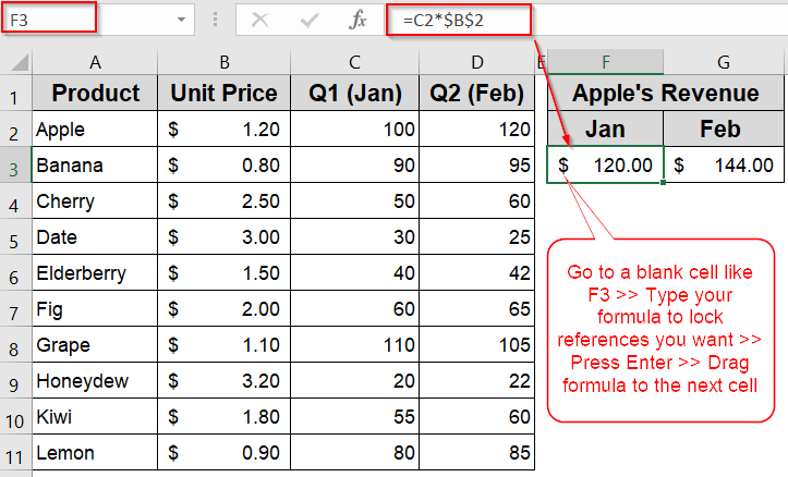
Steps to use mixed cell reference in Excel:
➤ Select a blank cell like F3.
➤ Use this formula: =C2*$B$2
Here, C2 is a relative reference, so it changes as you move across columns to pull monthly sales data and $B$2 is an absolute reference, meaning it keeps both the column and row fixed to always refer to Apple’s price.
➤ Press Enter.
➤ Drag the fill handle to the next cell G3.
What is a Mixed Cell Reference in Excel?
In Excel, cell references are used in formulas to refer to other cells. There are three main types: relative, absolute, and mixed. A relative reference (like A1) changes both the column and row when you copy the formula to another cell. An absolute reference (like $A$1) keeps both the column and row fixed, no matter where the formula is copied.
A mixed cell reference, on the other hand, locks only one part of the reference either the row or the column. You use a dollar sign ($) before the part you want to fix. For example, $A1 keeps column A fixed but allows the row to change, while A$1 locks the row but lets the column shift. Mixed references are helpful when building formulas that should partially adjust as they’re copied across a worksheet.
Example of Using Mixed Cell References to Lock Columns or Rows in Excel Formulas
Mixed cell references help you lock either the column or the row in a formula, so when you copy or drag it across cells, part of the reference stays fixed while the other part updates automatically.
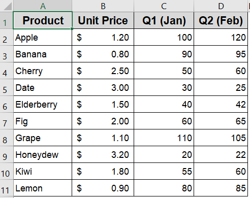
We will use a sample dataset containing 10 fruit products, their unit prices, and the number of units sold over two months (January and February). Our goal is to calculate monthly revenue by multiplying Price (column B) by the quantity sold for each month (columns C and D).
Steps:
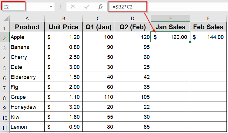
➤ Select cell C2.
➤ Enter this formula in E2 cell:
=$B2*C2
Here, $B2 locks column B, so it stays fixed when you drag the formula sideways. The row number 2 is relative, so it updates as you drag the formula down to different products and cell C2 is fully relative, so it changes both across rows and columns when copied.
➤ Press Enter.
➤ Drag the fill handle across to cell D2 (covering Jan to Feb).
➤ Then drag down from E2:F2 to row 11 to fill in all the products.
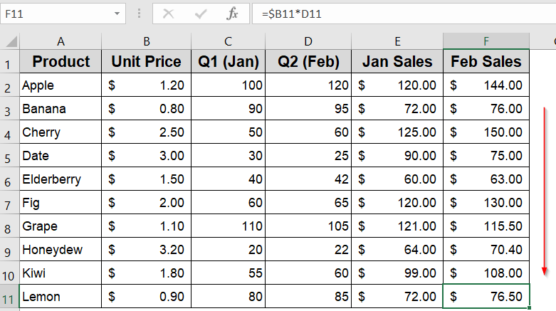
Now, columns E and F will show the correct monthly revenue for each product.
Example of Locking the Row with Mixed Cell Reference in Excel
When you want to keep the row fixed but allow the column to change as you copy a formula, you use a mixed reference that locks the row with a dollar sign before the row number (like $2).
In this example, we’ll calculate monthly revenue for Apple only by multiplying monthly sales by Apple’s price. As you drag the formula across months, the price reference will stay locked on Apple’s price row, while the sales column will update.
Steps:
➤ Select a blank cell like F3.
➤ Enter this formula:
=C2*$B$2
Here, C2 is a relative reference, so it changes as you move across columns to pull monthly sales data and $B$2 is an absolute reference, meaning it keeps both the column and row fixed to always refer to Apple’s price.
➤ Press Enter.
➤ Drag the fill handle to the next cell G3.
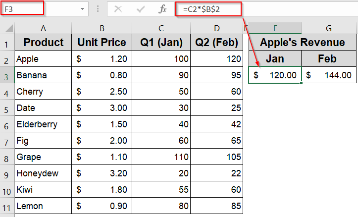
Now the cells from F3 and G3 now show Apple’s revenue by month.
Example of Using Mixed Cell References Inside Excel Functions Like SUMPRODUCT
Mixed cell references help you lock either rows or columns within functions so formulas adjust correctly when copied. This is especially useful for controlling lookup ranges or criteria in formulas like SUMPRODUCT function.
In this example, we’ll calculate total sales revenue by month, locking the price range while letting the sales range update as we drag the formula across columns.
Steps:
➤ Select a blank cell like F3.
➤ Enter this formula to calculate revenue for January (column C):
=SUMPRODUCT($B$2:$B$11, C$2:C$11)
Here, $B$2:$B$11 keeps both columns and rows fixed, so the price range doesn’t move and C$2:C$11 keeps the rows fixed but lets the column change when dragged sideways.
➤ Press Enter.
➤ Drag the fill handle to the next cell G3 to calculate the total revenue for Feb.
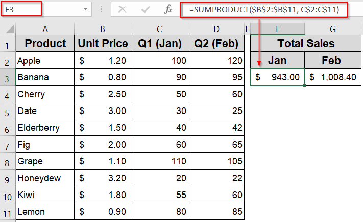
This shows total revenue for each month in F3 and G3 cells.
Example of Using Mixed Cell References to Calculate Total Pay with Bonus
When you need to calculate total pay including bonuses based on monthly sales, mixed cell references let you write a flexible formula that can be dragged down across rows. This method is useful when each employee has different sales and bonus percentages, and you want the calculation to update dynamically for each row.
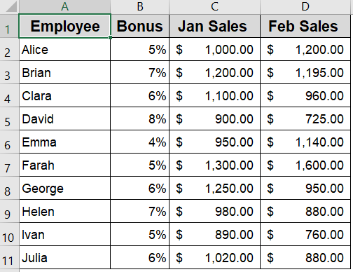
We’ll use a dataset containing employee names, their bonus percentages, and sales amounts for January and February. Our goal is to calculate total pay by summing the sales and then applying the bonus.
Steps:
➤ Select cell D2.
➤ Now enter this formula to lock the bonus percentage column but allow the row to change as you drag down:
=(C2 + D2) * (1 + B2)
Here, C2 + D2 adds the sales for January and February, while (1 + B2) scales the total by the employee’s bonus. The bonus cell B2 adjusts row-wise as you drag down, applying correctly for each employee.
➤ Press Enter.
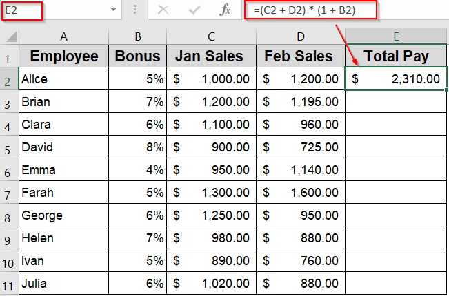
➤ Drag the formula down from E2 to E11 to fill for all employees
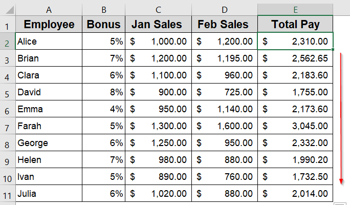
This method shows how mixed cell references adapt automatically to each row, giving accurate bonus-included totals without rewriting the formula.
Frequently Asked Questions
What is the difference between absolute, relative, and mixed cell references?
Absolute references (like $A$1) lock both row and column. Relative references (like A1) adjust completely when copied. Mixed references (like $A1 or A$1) lock either the row or the column only.
When should I use a mixed cell reference in Excel?
Use mixed references when copying formulas across rows or columns but you want either the column or row to remain constant. This helps maintain structure and prevents broken formulas when replicating calculations.
Can I convert a relative reference into a mixed reference easily?
Yes. While editing a formula, pressing the F4 key cycles through relative, absolute, and mixed references. This makes it easy to choose the right reference type without retyping your formula manually.
Why is my formula not working after copying across rows or columns?
If a formula gives incorrect results when copied, the issue may lie in the cell referencing. Use mixed references to lock either row or column and ensure only the necessary part adjusts during copying.
Is there a shortcut to apply mixed references in Excel formulas?
Yes. Select the cell reference in the formula bar and press F4 key. This cycles through all reference types such as relative, absolute, and mixed which allows you to quickly choose the right one for your formula.
Wrapping Up
In this tutorial, we explored multiple examples of mixed cell references work in Excel to lock either the row or column in a formula. We also saw how this technique helps maintain structure and accuracy when copying formulas across rows or columns. Whether you’re calculating revenues, bonuses, or totals, mixed references give you precise control over how Excel formulas behave. Feel free to download the practice file and share your feedback.