In Excel, applying conditional formatting based on another cell range means we format our selected cells using the values from other cells. During the process, you must use a suitable formula to determine which cells to format.
Steps to apply conditional formatting based on the matches of cells in two columns:
➤ Start by selecting the cell range you’re formatting. On the Home tab, navigate to the Styles group and click on Conditional Formatting.
➤ From the menu, select New Rule. Choose the Use a Formula to Determine Which Cells to Format option.
➤ In the Formula box, insert a formula based on what cell rule you want to apply. The following formula formats the cells of column D when they are equal to the corresponding cells in column C:
=$D2=$C2
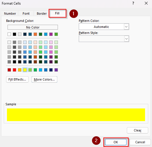
➤ Click Format, choose your formatting style, and press OK.
This article covers all the different formulas to apply conditional formatting based on another cell range for different cell rules such as equal to, greater than, less than, texts, and functions like AND, OR, and SEARCH.
Conditional Formatting Using the Equal to and Not Equal to Operators
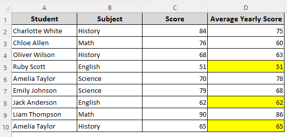
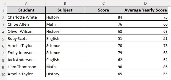
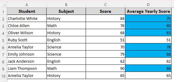
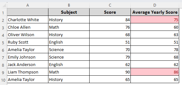
Our dataset features columns for student names and their obtained marks in different subjects. We’ll apply the conditional formatting rules mainly in column D based on the cell range of any other column.
In this example, we want Excel to format the cells of column D if the value in column D is (or is not) equal to the value in column C on the same row. Use it to highlight rows where two columns do or don’t match. Here are the steps:
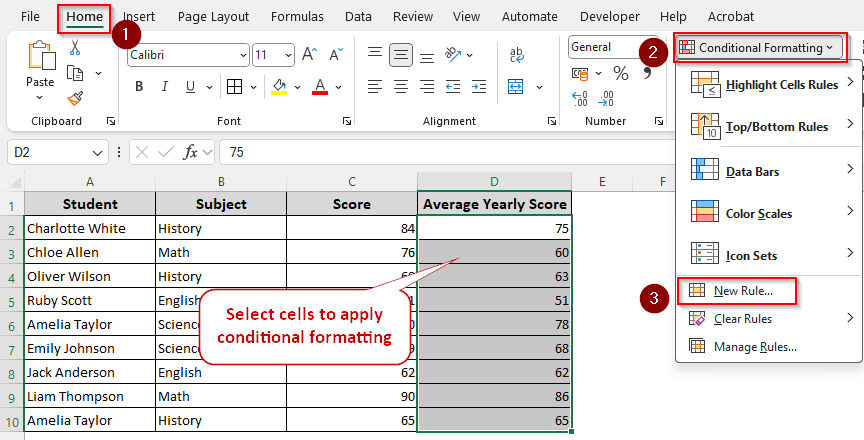
➤ Select the cell range where you want to apply conditional formatting rules. For non-adjacent columns or rows, press and hold the CTRL key and then select the ranges. We’re selecting the cells of column D.
➤ Go to the Home tab, select Conditional Formatting from the Styles group.
➤ Or, simply press the ALT + H + L shortcut keys to open it quickly. Choose New Rule from the drop-down menu.
➤ As the New Formatting Rule dialog box appears, select the Use a Formula to Determine Which Cells to Format option from the Select a Rule Type group.
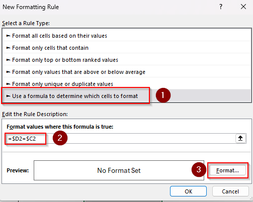
➤ In the Format Values Where This Formula Is True box, insert any of the following formulas:
To Apply the Equal to Operator
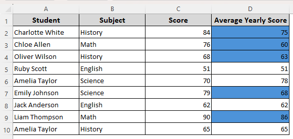
With this formula, we’ll check if the corresponding cells in Column C and D are equal. If yes, it will highlight the cells in column D containing similar values to column C.
=$D2=$C2

To Apply the Not Equal to Operator
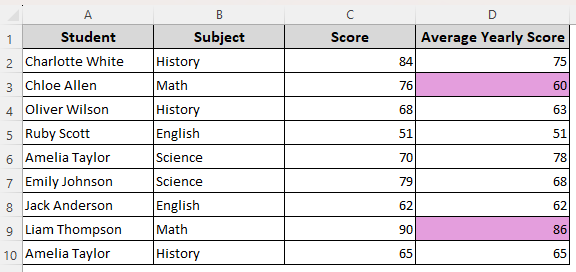
In this case, we’ll highlight the cells in column D that are not equal to the values of the same row in column C. All the cells of column D that fulfill this condition will be highlighted.
=$D2<>$C2
➤ Change the cell references according to your dataset.
➤ After entering the formula, click on Format and customize your formatting style by choosing a font, fill color, border, etc., from the Format Cells dialog box. Press Ok.
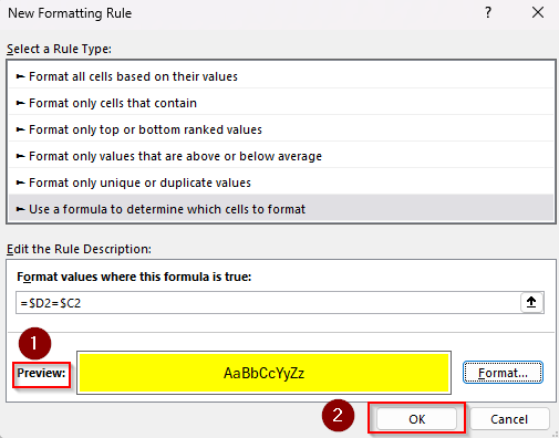
➤ Check out the Preview and press Ok to apply the conditional formatting rules.
Applying the Less Than and Greater Than Operators Based on Another Cell Range
Here, our goal is to format the cell(s) if it’s less than, greater than, less than or equal to, or greater than or equal to the corresponding reference cell range. For instance, we’ll highlight the cell D2 if the value in cell D2 is less than or greater than C2.
Using a relative or mixed formula will apply the same rule to the following cells of the selected range. Let’s get to the steps:
➤ Select the target range and go to the Home tab >> Conditional Formatting >> New Rule >> Use a Formula to Determine Which Cells to Format.
➤ In the formula box, enter any of the following formulas:
Using the Greater Than Operator
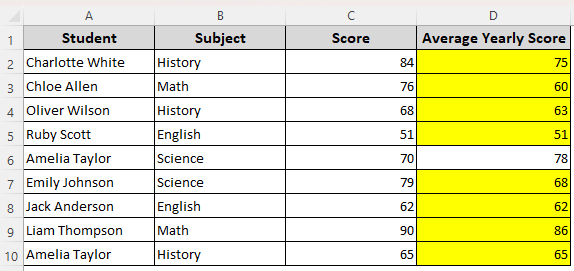
The following formula checks if the values of column C are greater than the values of the same rows in column D. If yes, Excel will highlight those cells in the same row in Column D.
=$C2>$D2
Using the Greater Than or Equal To Operator
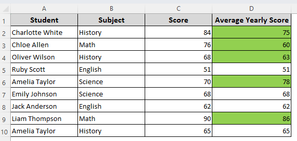
Here, our formula checks whether the values in column C are greater than or equal to the values of corresponding cells in column D. Any cell in column D that meets either of the conditions is highlighted.
=$C2>=$D2
Using the Less Than Operator
We use the following formula to find and highlight values in column D that are greater than the values of column C in the same row.
=$C2<$D2
Using the Less Than or Equal To Operator
Now, we’ll check if the values in column D are greater than or equal to the values in the corresponding cells of column C. This formula will format the cells in column D meeting at least one of the given conditions.
=$C2<=$D2
➤ Click on Format to apply format styles and press Ok.
Cell Rules for Texts Based on a Selected Cell Range
Let’s learn about cell rules for texts including highlighting corresponding cells based on a fixed text, parts of a text, and multiple texts. We’ll select a text from column B and apply formatting to the corresponding cells of column D. Here’s how:
➤ Select the cells where you want to apply the conditional formatting rules and click on Home >> Conditional Formatting >> New Rule >> Use a Formula to Determine Which Cells to Format.
➤ Enter any of the following formulas in the formula field:
Highlight Cells Corresponding to Single Text
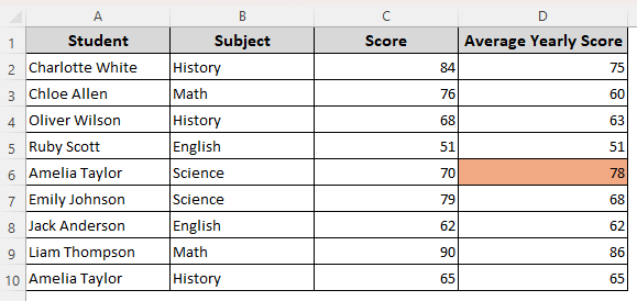
With the following formula, we’ll look for the text Math in column B. If found, conditional formatting will be applied in the corresponding cell of column D.
=$B2=”Math”
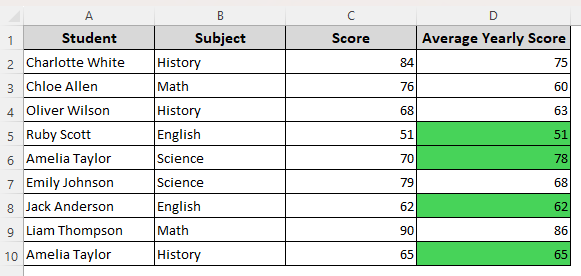
Highlight Cells Corresponding to Multiple Texts
Our goal here is to look for multiple texts such as Math, English, and History. Adding the OR function allows us to highlight corresponding cells in column D when any of these texts are found in column C.
=OR($B2=”Math”, $B2=”English”, $B2=”History”)
Highlight If Text Isn’t Found in the Fixed Range
Use the following formula to find all the values in column D that don’t match the values in column D. Conditional formatting rules highlight the cells of column D not matching the values of the same rows in column C.
=ISNA(MATCH(D2, $C$2:$C$10, 0))
➤ Change the cell reference and texts based on your dataset.
➤ Click on Format and select your preferred highlighting options. Press Ok.
Applying Multiple Conditions Using the AND and OR Functions
In this case, we’ll format cells only if multiple conditions are met. For instance, we’ll highlight cells in column D if the corresponding cells in column B contain a certain text (Math) and/or column C contains a value greater than a certain number (80). Here are the steps:
➤ Choose the cells for formatting and open the Home tab >> Conditional Formatting >> New Rule >> Use a Formula to Determine Which Cells to Format.
➤ Insert any of the formulas given below in the designated field for formula:
Format When All Conditions Are True
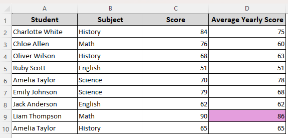
Here, we’re looking for the text Math in column B and all the values in column C greater than 80. Only when both conditions are found in the same row, Excel highlights the corresponding cell in column D.
=AND($B2=”Math”, $C2>80)
Format When At Least One Condition Is True
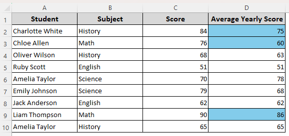
In this case, we’re also looking for certain texts and values in columns B and C. However, unlike the previous formula, this one highlights the cells of column D if any of the given conditions are found in the same row.
=OR($B2=”Math”, $C2>80)
Applying Conditional Formatting Based On Another Cell Range Using VBA Coding
With VBA coding, we can create a custom VBA macro that formats cells based on the cell rule you define. This macro allows you to apply any formula you want to set conditional formatting rules. For our dataset, we’ll check which cells of column C are greater than 80.
If the condition is met, the macro will highlight the corresponding cells in column D. Below are the steps for it:
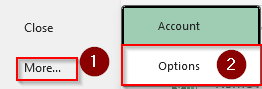
➤ To add the Developer tab on Excel’s main ribbon, go to the File tab >> More >> Options.
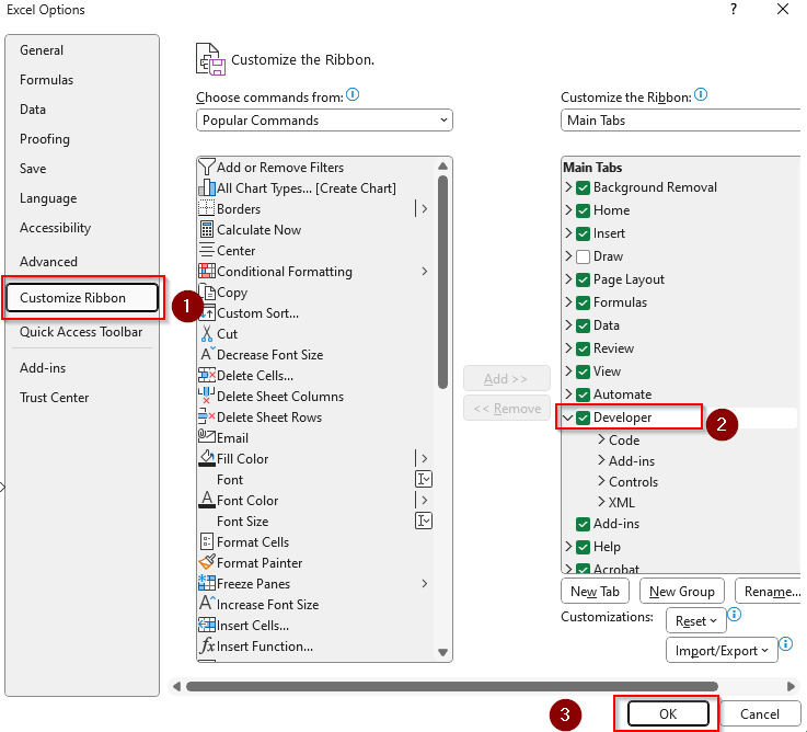
➤ Choose Customize Ribbon from the side column and check the Developer option. Click Ok.
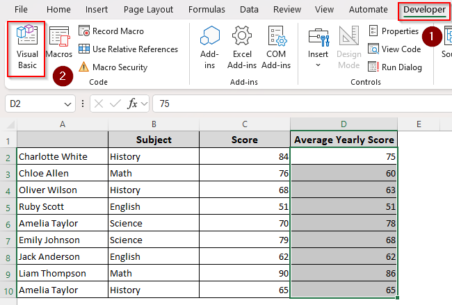
➤ Select your cell range to apply conditional formatting. Go to the Developer tab and click on Visual Basic.
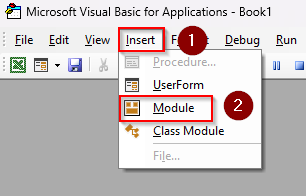
➤ In the VBA Editor, select Insert from the top ribbon and choose Module from the drop-down menu.
➤ Paste the following code in the blank Module box:
Sub ApplyConditionalFormattingFromUserFormula()
Dim formula As String
Dim selectedRange As Range
Dim ws As Worksheet
' Prompt the user to enter a formula
formula = InputBox("Enter the conditional formatting formula (e.g., =A1>100):", _
"Conditional Formatting Formula")
' Exit if the formula is empty
If formula = "" Then
MsgBox "No formula entered. Operation cancelled.", vbExclamation
Exit Sub
End If
' Set the worksheet and selected range
Set ws = ActiveSheet
On Error Resume Next
Set selectedRange = Application.Selection
On Error GoTo 0
' Check if selection is valid
If selectedRange Is Nothing Then
MsgBox "Please select the cells where you want to apply the formatting.", vbCritical
Exit Sub
End If
' Clear any existing conditional formatting
selectedRange.FormatConditions.Delete
' Add the new conditional formatting rule
With selectedRange.FormatConditions.Add(Type:=xlExpression, Formula1:=formula)
' Example formatting: light red fill with dark red text
.Interior.Color = RGB(255, 199, 206)
.Font.Color = RGB(156, 0, 6)
End With
MsgBox "Conditional formatting applied based on your formula.", vbInformation
End Sub
➤ Press F5 or click on the Run tab from the top ribbon and choose Run Sub/UserForm.
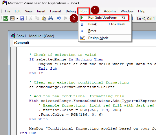
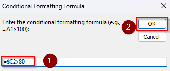
➤ Now, in the Conditional Formatting Formula box, enter a formula to fix a cell rule. You can use any of the formulas discussed above or use a different one according to your needs. Press Ok and the formatting will be applied.
➤ Before closing the tab, make sure you save the file when Excel prompts you to save it in the correct format. Here’s our final result:
Frequently Asked Questions
Can I use an IF function in conditional formatting?
Yes, you can use the IF() function in conditional formatting. However, IF() returns a value (not just TRUE or FALSE), which can be messy in conditional formatting. Therefore, you need to use it in a formula in the following way:
=IF(B2=”Math”, TRUE, FALSE)
Change the A2=”Math” argument as needed.
How do you conditionally format a cell based on a date in another cell?
Let’s say you want to format D2:D10 if A2:A10 has a date before today. Select D2:D10 and open the Conditional Formatting dialog box and enter the formula given below:
=$A2<TODAY()
Change the cell references and the formula arguments as needed.
How to create conditional formatting based on another range for blank cells?
To highlight column D (D2:D10) if the corresponding cell in column A is blank, enter the designated field in the following formula in the conditional formatting dialog box:
=$D2=””
You can also use the following formula to highlight non-blank cells:
=$D2<>””
Concluding Words
Essentially, using the conditional formatting option with a formula and creating a VBA macro are the two ways of applying conditional formatting based on another cell range in Excel.
In both cases, you must use the correct formula that formats cells based on whether the given argument is true or false.