Autofill form in Excel is a powerful tool that can be customized to let organizations manage deadlines, monitor task progress, track employee assignments and streamline reporting processes. By using Excel’s built-in tools, users and organizations can easily create their own structured, user-friendly interface to input and store data directly into a spreadsheet file.
Follow the steps below to create your very own autofill form using Excel:
➤ First, set up your dataset with clear column headers. Make sure the headers are properly structured and easy to interact with.
➤ Then, format the dataset with borders, colors and add necessary elements like input fields, checkboxes and dropdown menus.
➤ Create a separate Data sheet to store the submissions and link it to the main form.
➤ Next, record a Macro that automates the form submission process by storing the form entries in the Data sheet.
➤ Add a submit button tied to the macro to confirm form submission.
➤ Lastly, hide the helper rows and protect the sheet to prevent accidental changes
In this article, we will learn how to create an autofill form in Excel by following nine simple steps.
Step-by-Step Guide to Creating an Autofill Form in Excel
Creating an autofill form in Excel might seem challenging at first, but by following a proper step-by-step guide, the process becomes simple and effective. Follow the steps below to successfully build your own Autofill Form in Excel.
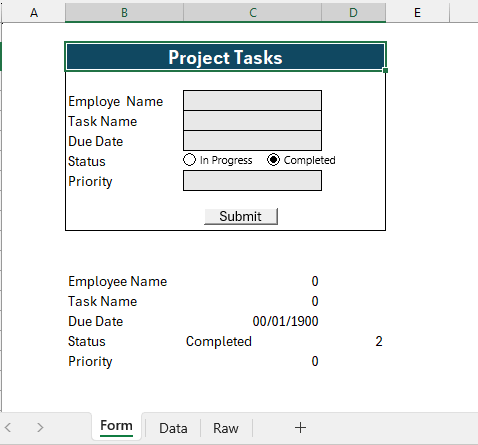
Step 1: Format the Form Sheet
➤ Open Excel and create a new worksheet called Form.
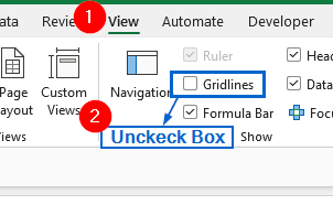
➤ Hide gridlines by heading to View >> uncheck Gridlines.
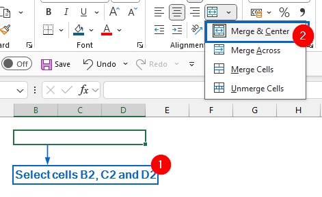
➤ Select cells B2 to D2, merge them into a single cell.
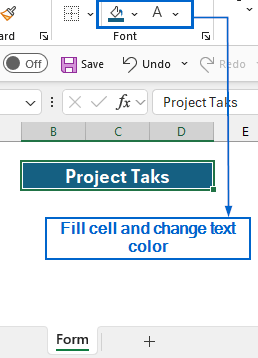
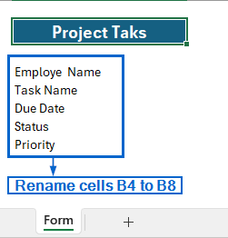
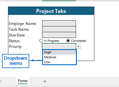
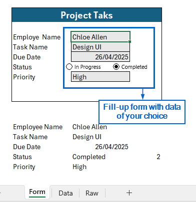
➤Then, fill the cells with a deep blue color, set the text color to white, and label the merged cell as “Project Tasks”.
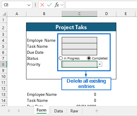
➤ Select cells B4, B5, B6, B7 and B8, label them as Employee Name, Task Name, Due Date, Status and Priority, respectively.
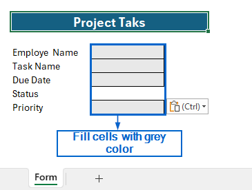
➤ Again, select cells C4, C5, C6, and C8 and fill them with grey color by heading to Home >> Fill Color from the main menu.
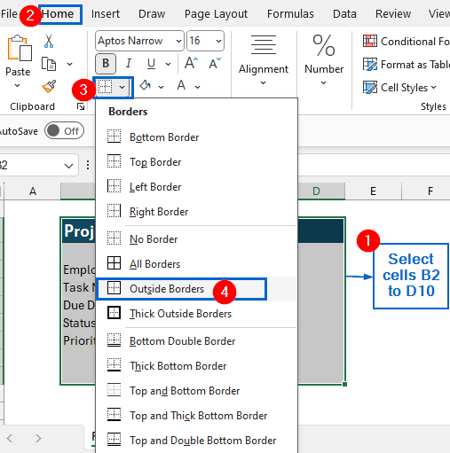
➤ Last of all, select cells B2 to D10 and from the main menu go to Home >> Borders >> Outside Borders to add an outside border and make the form more visually organized.
Step 2: Add a Checkbox for the Status Label
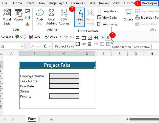
➤ Head to Developer tab from the main menu. Then select Insert >> Option Button.
Note:
If the Developer tab is not visible, head to the main menu, right-click your mouse and select Customize the Ribbon option. From Customize the Ribbon menu, check the box before Developer and click on OK.
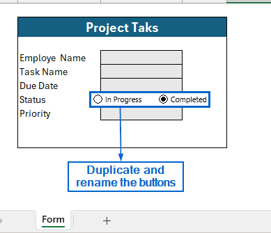
➤ Place the option button right next to the Status label in Project Tasks form.
➤ Press Ctrl + C and Ctrl + V , duplicate the button and rename them to “In Progress” and “Completed”.
Note:
To rename the buttons, right-click on them and choose Edit Text.
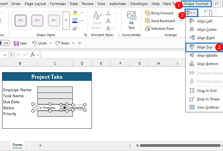
➤ Next, select both buttons and go to Shape Format from the main menu. From there, click on Align>> Align Top. Both your buttons should be perfectly aligned with the Status label now.
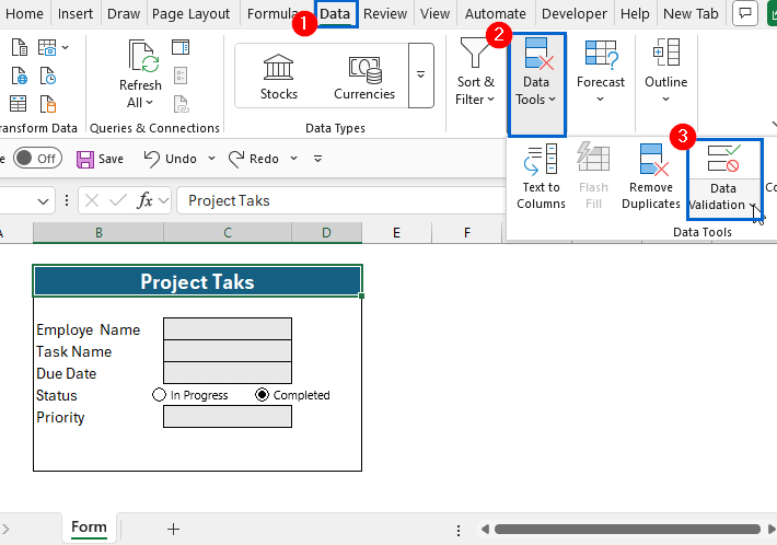
Step 3: Create a Dropdown for Priority Label
➤ Now, select cell C8 and head to Data >> Data Tools >> Data Validation.
➤ From the Data Validation menu, set Allow to List and type High, Medium, Low in the Source option.
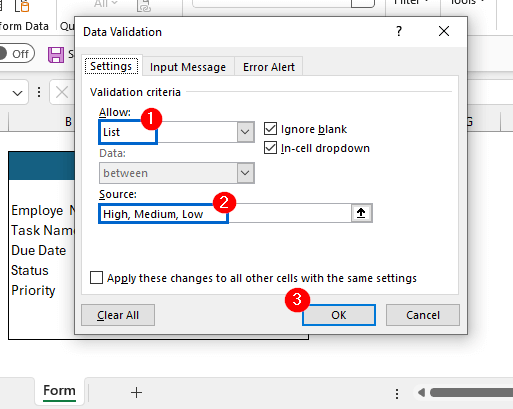
➤ Click on OK to create a dropdown menu in cell C8.
Step 4: Add a Helper Row for Data Processing
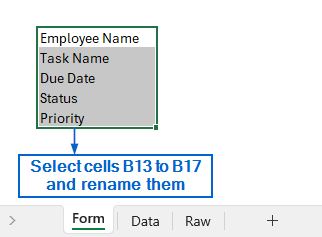
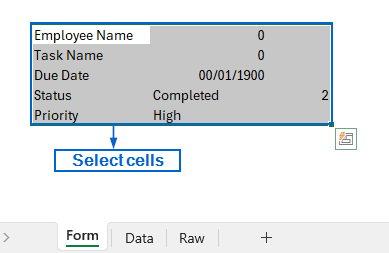
➤ In the Form worksheet, select cells B13 to B17 and rename them as Employee Name, Task Name, Due Date, Status and Priority, respectively.
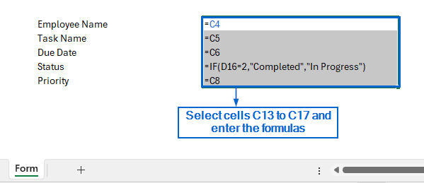
➤ Now, select cells C13 to C17 and link each of them to the corresponding form input fields by entering the following formulas:
➧ C13:=C4
➧ C14:=C5
➧ C15:=C6
➧ C16:=IF(D16=2,”Completed”,”In Progress”)
➧ C17:=C8
Note:
These formulas will automatically pull data from the form inputs and display them in the linked cells of the helper row.
Step 5: Create a New Worksheet to Display Form Data
➤ Now, create a new worksheet named “Data”.
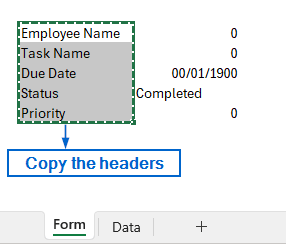
➤ Next, head to the Form worksheet and copy the headers from the helper row (cells B13 to B17).
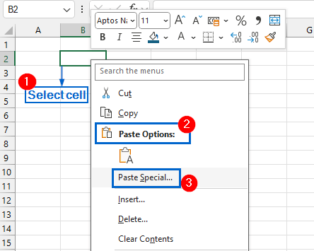
➤ Again, head to the Data worksheet, select cell B2, right click your mouse and from Paste options select Paste Special.
➤ In the Paste Special menu, select Values from the Paste option and check the Transpose box.
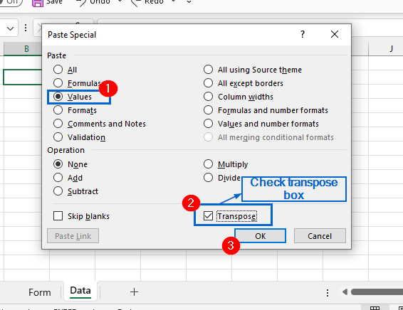
➤ Click on OK to finish copying the headers to Data sheet from the Form sheet.
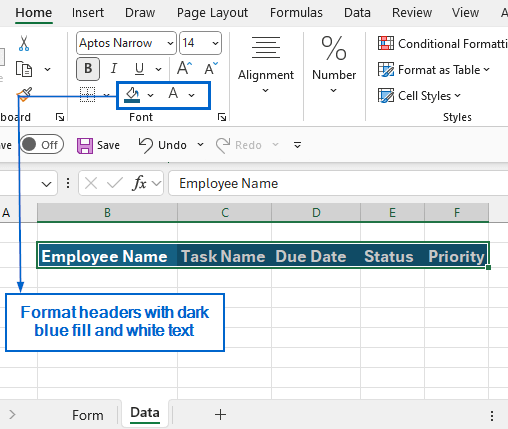
➤ Finally, format the header cells with dark blue fill and white font color.
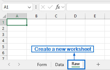
Step 6: Create a Raw Data Sheet
➤ Create a new empty worksheet called “Raw”
Note:
This sheet will temporarily hold transposed data from the Form worksheet during the automation.
Step 7: Record a Macro to Automate the Process
➤ Head to Form worksheet and fill in the form fields with Data of your choice.
➤ Next, head to the Developer tab and click on Record Macro button.
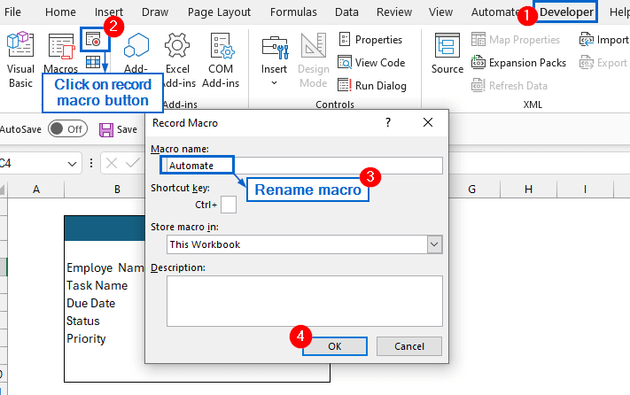
➤ Rename the macro to Automate and click OK.
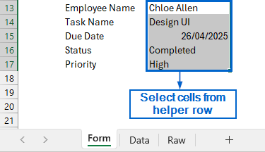
➤ Now, head to the helper row and copy all contents from cells C13 to C17.
➤ Go to the Raw worksheet, select cell A1, right click to bring out Paste options and select Paste Special.
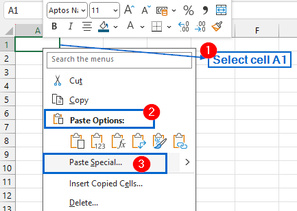
➤ Just like Step 5, in the Paste Special menu, select Values from the Paste option and check the Transpose box.
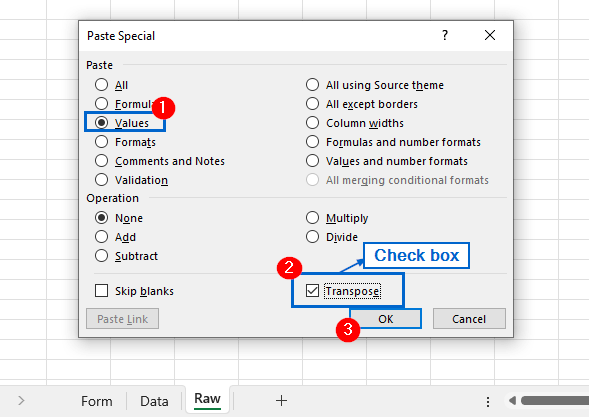
➤ Click on OK to paste all headers from the Form worksheet to Raw worksheet.
Note:
To ensure dates are displayed correctly, format column C by right-clicking the column header and heading to Format Cells >> Date.
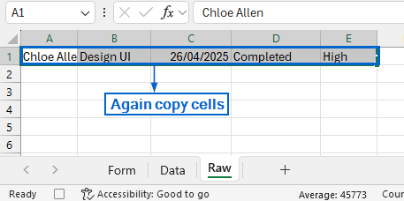
➤ In the Raw worksheet, again copy all contents from cell A1 to E1.
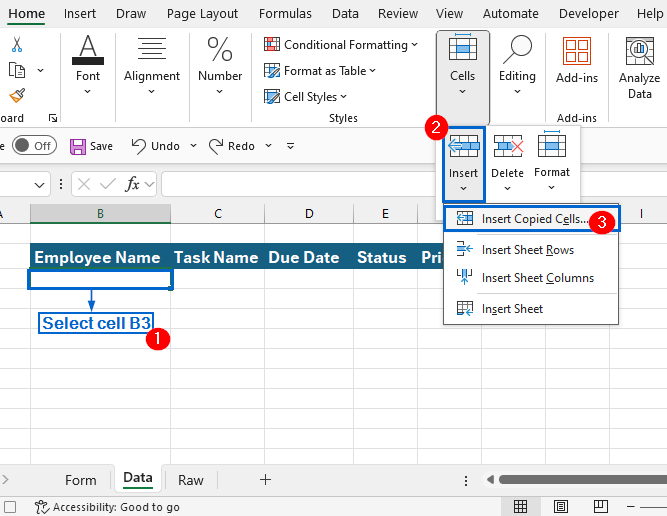
➤ Head to Data worksheet, select cell B3, and from Home tab go to Insert >> Insert Copied Cell.
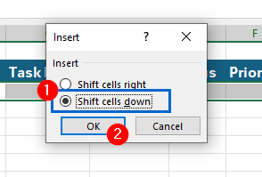
➤ From the dialogue box, check Shift cells down option and click on OK.
➤ Again, head to Form worksheet and delete all the existing entries from the form.
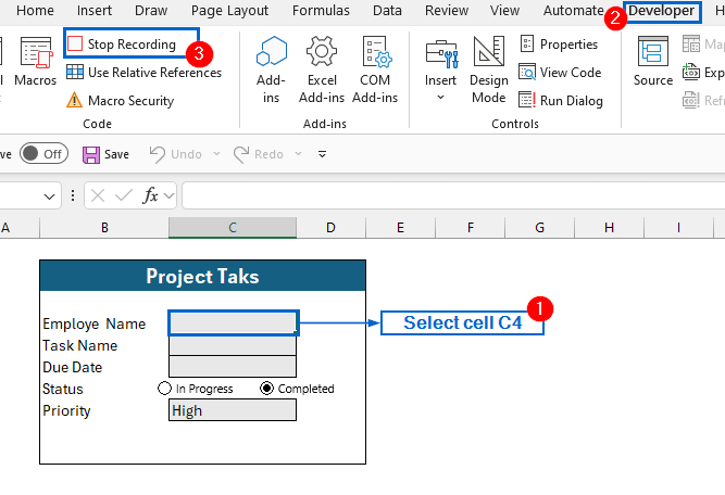
➤ Now, select cell C4, head to the Developer tab and click on Stop Recording. You have now successfully recorded the macro.
Step 8: Add a Submit Button
➤ In the Form worksheet, head to the Developer tab, click on Insert >> Button.

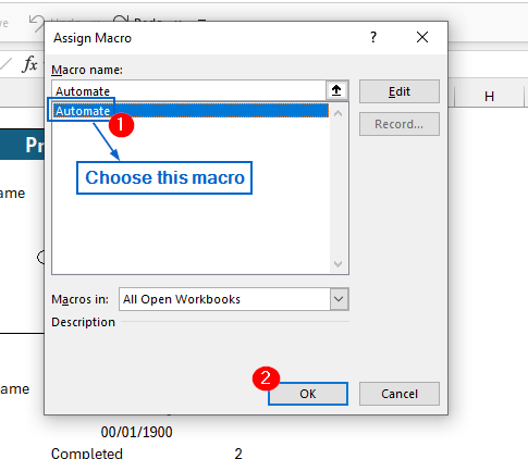
➤ Draw the button below the form and rename the macro to Automate from the Assign Macro dialogue box. Click on OK to finish assigning the button.
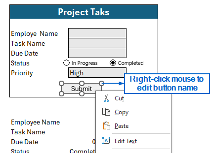
➤ Rename the button to Submit by right-clicking on it.
Step 9: Hide the Helper Row
➤ Again, head to Form worksheet. Select cells B13 to D17.
➤ Then, head to Home tab and change the text color to white.
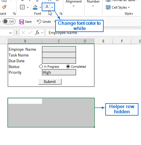
Note:
Changing text color to white will effectively hide the helper row by blending it with the background.
Now, when you fill out the form with relevant data in the Form worksheet, the entries will automatically appear in the Data worksheet.
Frequently Asked Questions
What are Helper Rows and Why are They Needed?
Helper rows are hidden rows in Excel that are used to temporarily store data. They ensure that the data is properly organized, formatted, and ready to be transferred when the macro is triggered. Without helper rows, automating the data submission process becomes more complex and difficult.
Can I Edit the Form Layout After Creating it?
Yes, you can make changes to the form layout after creating it. You can also alter color and positioning of elements even after the form is functional. Just make sure the formula references and macro steps are updated accordingly.
Why is the Submit Button On My Form Not Working?
If your submit button is not working, then there is most probably an error or misconfiguration in the recorded macro. Make sure that the macro is properly recorded and the button is correctly assigned to the recorded macro.
Concluding Words
Autofill form in Excel helps reduce data entry time, ensures consistency, and improves accuracy in your spreadsheets. In this article, we have discussed how to autofill a form in Excel by using nine simple steps. Feel free to practice the steps and create your own custom form depending on your needs.