Excel frequently requires working with data from multiple sources across several different worksheets. At times, you might need to pull data from multiple worksheets into one single worksheet to keep record of it. Now, it is possible to manually copy and paste data from every sheet. However, this process is extremely time consuming and prone to mistakes when you are handling big sets of data. Excel has a number of strong tools and features that let users effectively pull data from various spreadsheets into a single sheet.
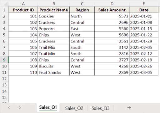
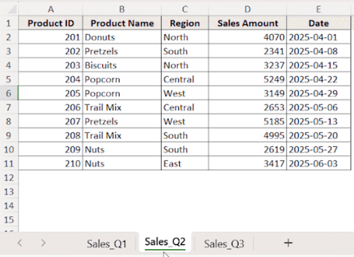
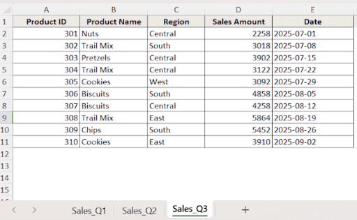
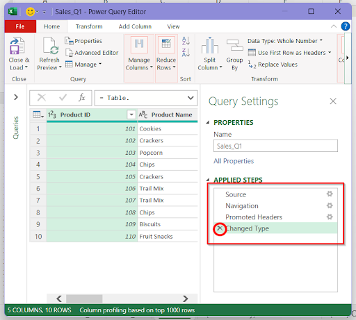
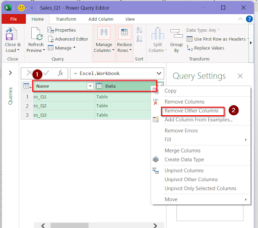
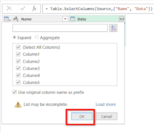
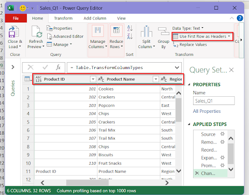
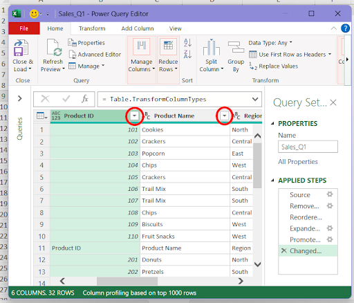
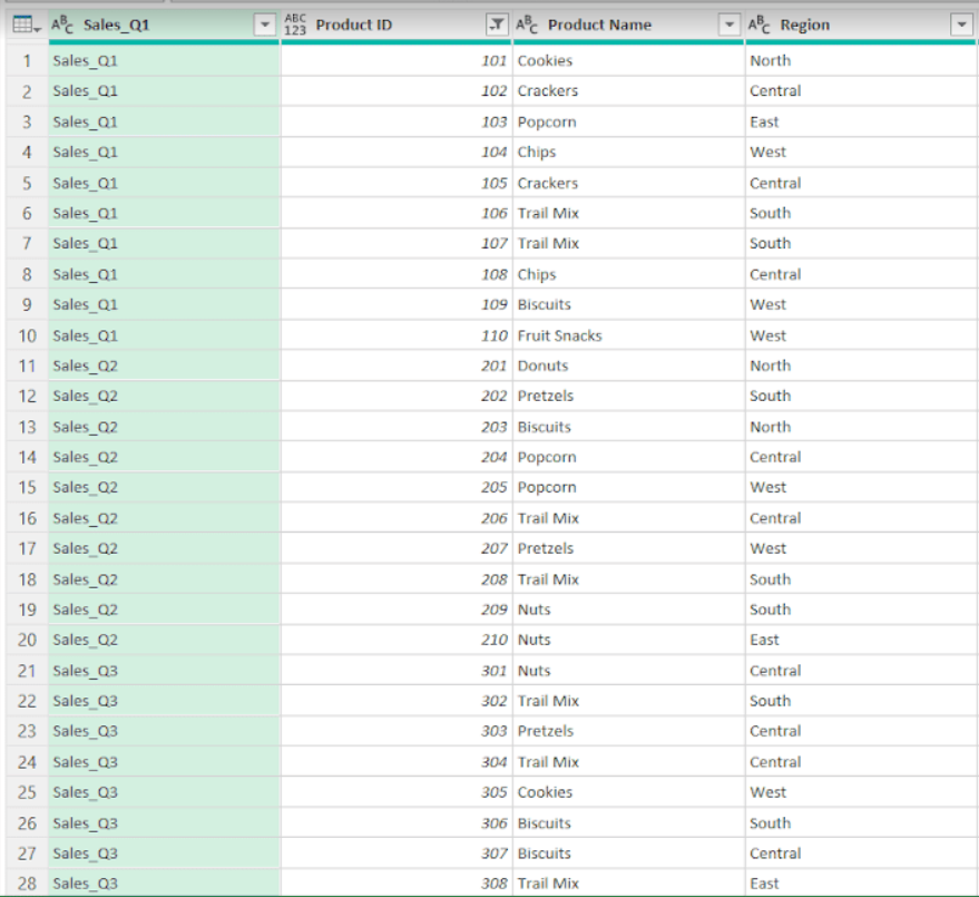
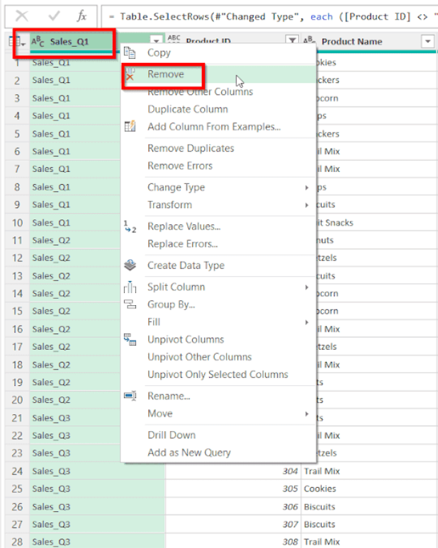
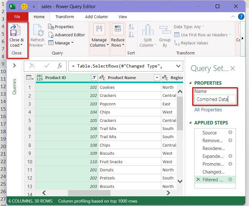
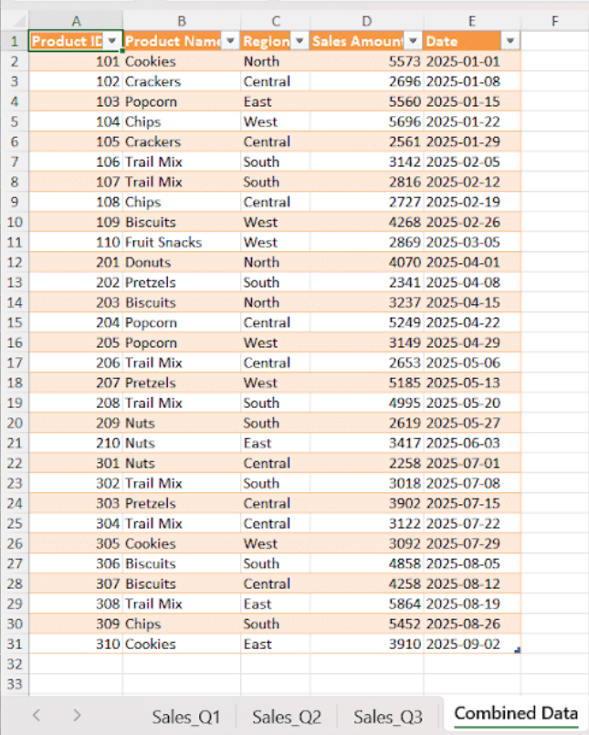
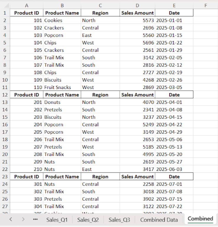
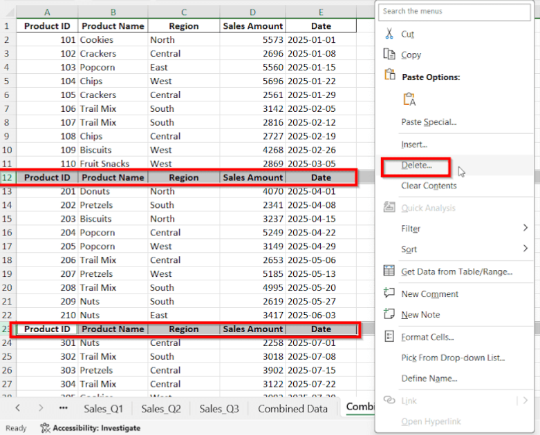
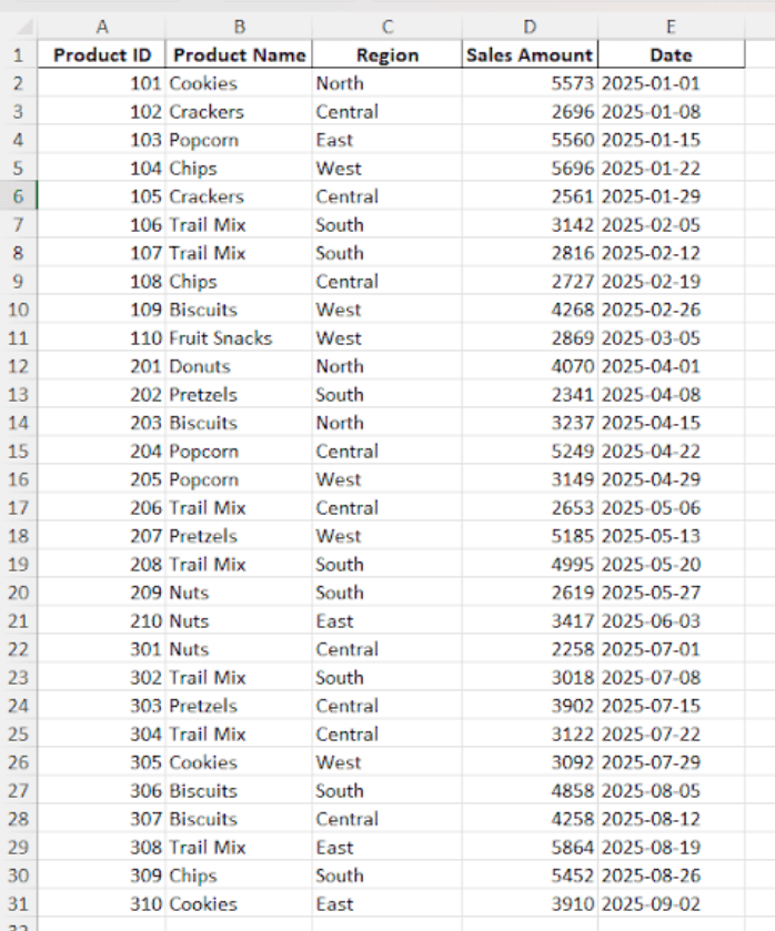
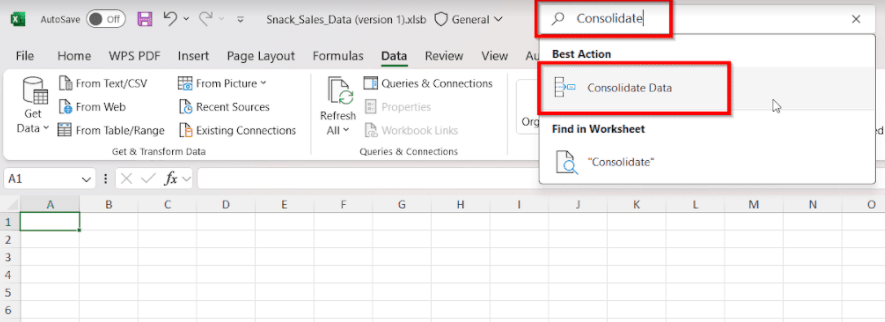
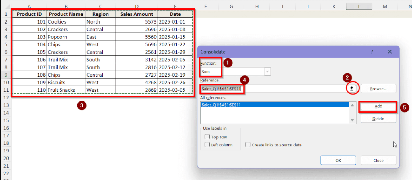
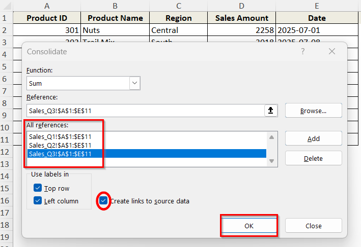
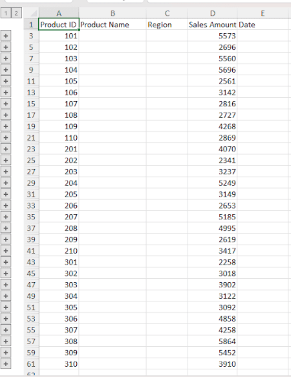
➤ Select Get Data > From File > From Excel Workbook to access the sheets you want to pull data from. We’ll show you how to pull data from multiple worksheets by using power query, VBA code and the Consolidate feature with every detailed step in this guide. This will help you operate more efficiently in Excel, save time and reduce mistakes. Power query is the best option for collecting data from several sheets as it perfectly combines both numerical and non-numerical data into a new worksheet. Suppose, we have these three different worksheets containing the snack sales of a company at different locations. Here’s the first one- The second one- And the third one- Now, we will follow the steps below in order to pull all these data into a single worksheet by using Power Query- ➤ Select the workbook containing your needed sheets from the files. Click on Import next. ➤ A navigator box will pop up where you need to click on the corner to show all the sheets. ➤ At the top left, tick the Select multiple items box first. Now, individually tick on all the sheets you want to combine. Here, we want to combine all three worksheets so we have clicked the tick boxes of all three. ➤ The tables will show up individually in the Power Query Editor too. So, at the right bar under Applied Steps options, we will click the cross beside all the options except the Source. ➤ Press CTRL + ALT and select the columns Name and Data. Right click and choose Remove other columns. Now, you will be left with only the worksheets and their data. ➤ Click on the corner of the Data column to expand it. ➤ All the columns in the expanded box will already be ticked so just press OK. The data from all the worksheets will now be compiled into a single table. ➤ From the Home tab, select the option Use First Row as Headers. ➤ Now, you can see a repetition of the header row from worksheet 2 and 3 in the table which we need to remove. For that, we need to use the filter option beside any of the header as shown in the picture. ➤ For example, click on the expand button next to the header Product ID. Scroll down the filter section and untick the box beside Product ID as it should only show up once as the header. Then click OK. ➤ Now, all the repetitive header rows will disappear from the entire table. You can do this on any of the header options and it will give the same result. ➤ We don’t want the source worksheet to be shown on the first column as it is now. So, right click on the Sales column and click on Remove to get rid of it. ➤ You can name the query as you want from the right side Properties box. We have named it Combined Data. ➤ Now, you can click on Close & Load and all the combined data from multiple worksheets will now be shown on one single worksheet. The next method we are going to see is the use of a VBA code to extract the data into a single worksheet. For this method to work, make sure all the source worksheets have similar structures such as the same headings, same order of columns and rows. Now, you can do this by following these simple steps– ➤ Open your Excel workbook and press the Alt + F11 and it will open the window Microsoft Visual Basic for Applications. ➤ Copy this VBA code. Right click and select Paste into the Module window. VBA Code for combining data: ➤ Click on Run or alternatively press F5 to run the code. ➤ Now, all data from the worksheets have been gathered in a single worksheet as “Combined”. ➤ Select the repetitive header rows in this sheet and delete them to only have one header in the 1st row. ➤ All the data from three worksheets will now be compiled perfectly into one worksheet. The Consolidate feature of Excel is a great help in combining data but it comes with some limitations. The biggest drawback of this method is that it will only combine and merge the numerical data from the worksheets. Let’s take a look at how this method works- ➤ Open a new worksheet and in the search bar, type in Consolidate to select the feature. ➤ In the box, select the function as SUM. In the reference box, select each of the tables from multiple worksheets that you want to combine. After selecting each, click on Add beside the reference box. ➤ Once you’re done selecting and adding all the tables to the All References box, click OK. ➤ Only the numerical data will be pulled from all the worksheets. The textual and non numerical data like the dates, product name or region will be absent this way. ➤ Now, you will need to manually copy and paste the missing non numerical data from the worksheets if you need them. So, this is a hassling method to merge data and it is not recommended. In the Power Query method, you can pull data from different worksheets stored in different workbooks very easily. All you need to do is use the Get Data > From Files > From Excel Workbook option and select the separate workbooks you need to combine from there. No, the Consolidate feature in Excel is very convenient when it comes to merging and combining numerical values and data from separate worksheets. However, this feature can’t pull textual and non numerical data and combine them which is very troublesome since most worksheets have at least one column of non numerical data. It also can’t combine date formats. There is no way to directly use the Consolidate feature and combine textual data into a single worksheet. The feature will only combine the numerical values onto the worksheet. Afterwards, you will need to manually copy paste the non numerical columns or rows separately in the new worksheet. If you are using Power query for this, you can easily update the combined worksheet when new data is added to the source worksheets. Go to Data > Refresh All to update the data instantly in the merged worksheet. So, pulling data from multiple worksheets in Excel does not have to be time consuming or too difficult. With these methods covered in this article, you can accurately combine data from various worksheets within minutes. The Power Query and VBA code are the two best methods for this which works for all kinds of numerical and non numerical data. On the other hand, the Consolidate feature is really not recommended while dealing with non numerical data. Let us know which method worked the best for you!
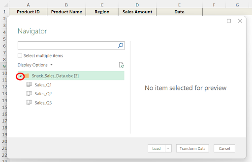
➤ In the Navigator, tick Select multiple items, tick the sheets and click Transform Data.
➤ In Power Query Editor, remove extra columns or repeated headers using filters and combine data into a table.
➤ Click Close & Load to create a new spreadsheet containing all data from multiple sheets. 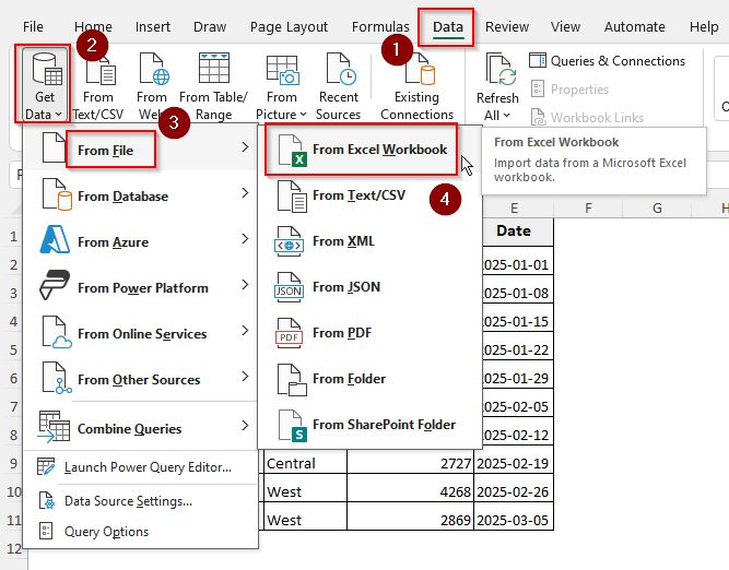
Use Power Query to Pull Data From Multiple Worksheets into One Sheet
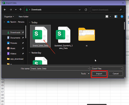
➤ First, open the workbook containing all the sheets you want to combine.
➤ Create a new sheet which is completely empty. We will combine the data in this new sheet. You can rename this sheet according to your needs.
➤ Now, go to the Data tab from the ribbon. Click on Get Data > From File > From Excel Workbook. 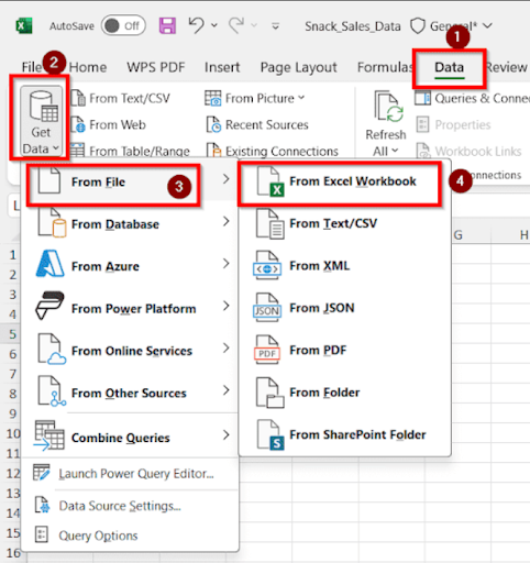
➤ Each of the sheets will be previewed at the right side of the box. If you are done selecting, select Transform Data which will open up the Power Query editor. 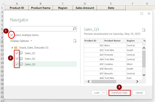


Use a VBA Code to Pull Data from Multiple Worksheets into One Sheet
➤ From the tabs, click on Insert > Module. An empty module window will open up. 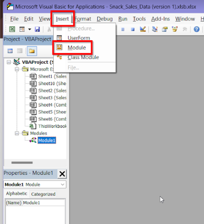
Sub Combine()
'UpdatebyExtendoffice20180205
    Dim I As Long
    Dim xRg As Range
    On Error Resume Next
    Worksheets.Add Sheets(1)
    ActiveSheet.Name = "Combined"
   For I = 2 To Sheets.Count
        Set xRg = Sheets(1).UsedRange
        If I > 2 Then
            Set xRg = Sheets(1).Cells(xRg.Rows.Count + 1, 1)
        End If
        Sheets(I).Activate
        ActiveSheet.UsedRange.Copy xRg
    Next
End Sub 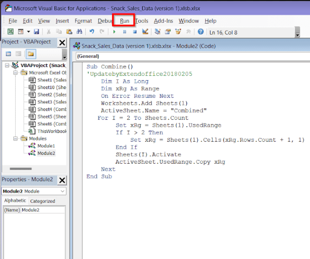
Use Consolidate Feature to Pull Data from Multiple Worksheets
FAQs
Can I Pull Data from Multiple Workbooks into One Worksheet?
Can Consolidate Feature Combine All Types of Data into a Single Worksheet?
How Can I Pull Non Numerical Data Using Consolidate Feature?
Can I Automatically Update the Combined Worksheet When the Source Worksheets Are Changed?
Wrapping Up