
When we work with spreadsheets, it is a common thing that we need to extract text after a certain character. Only part of the data within a cell. For example the text after a specific character like a comma, dash, or symbol or even alphabets. Whatever your dataset is, if you are cleaning up imported data or maybe handling email addresses you need to know this text extraction technique. It can save hours of your manual work.
To excel extract text after character, follow these steps:
➤ Select the cells containing the text.
➤ Use a formula such as =RIGHT(B2, LEN(B2) – SEARCH(“@”, B2))
➤ Press Enter and copy the formula down the column to fill the whole column.
In this article, you will learn multiple methods to extract text after a character in Excel. We will do that by MID with FIND, RIGHT, using the built-in Text to Columns tool and more.
Using MID, FIND, and LEN Functions to Extract Text After Character
The MID function combined with FIND (or SEARCH) and LEN is a good way to extract text that appears after a specific character in a string. We usually use it when we are dealing with datasets like product codes, names, or identifiers and where our desired text is always after a specific symbol (like a hyphen).
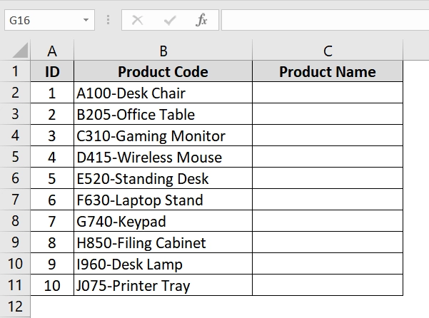
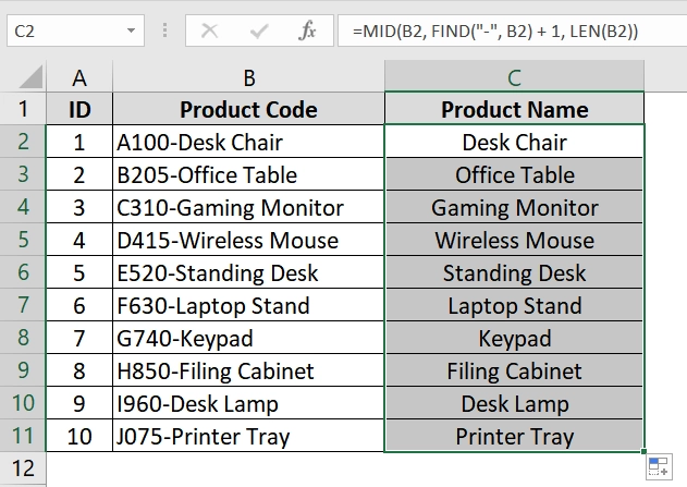
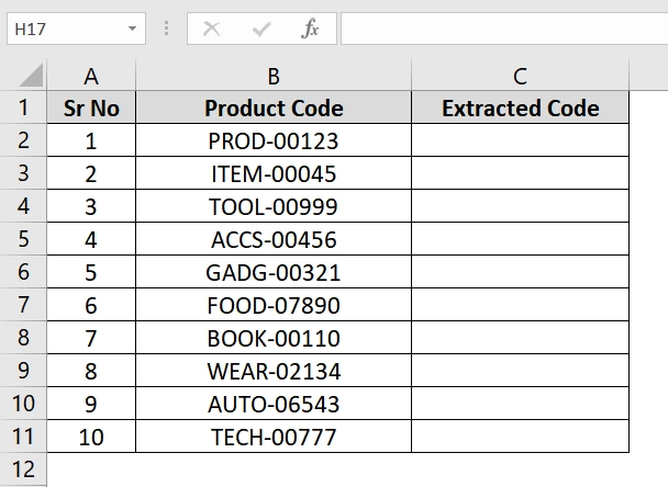
Here we have a dataset where we have some code and then hyphen and then name of some product and we want to extract the product name which is always after the hyphen sign.
Steps:
➤ Opet up your dataset. In our dataset the product codes (e.g., A100-Desk Chair) are in Column B, starting from cell B2.
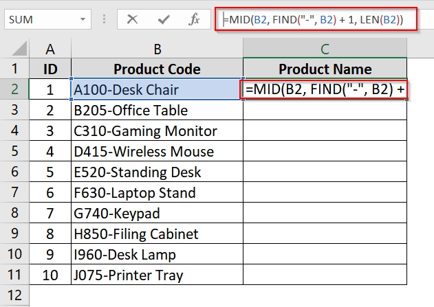
➤ Click on cell C2, where you want to extract the product name (text after the hyphen).
➤ Enter the following formula:
=MID(B2, FIND(“-“, B2) + 1, LEN(B2))
Here,
- FIND(“-“, B2) locates the position of the hyphen.
- +1 ensures the extraction starts after the hyphen.
- LEN(B2) gives the total number of characters from which the MID will start extracting until the end.
➤ Press Enter to see the extracted product name.
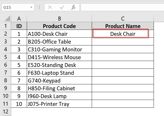
➤ Use the fill handle to drag the formula down the column and apply it to the rest of the rows.
Note:
➧ If your delimiter is different (e.g., comma or colon), replace “-” with the appropriate character.
➧ You can use SEARCH instead of FIND if you are not sure about case sensitivity. SEARCH is case insensitive.
➧ If there is no delimiter in the cell, the formula will return an error. Use IFERROR for a cleaner result: =IFERROR(MID(B2, FIND(“-“, B2) + 1, LEN(B2)), “”)
Applying RIGHT, LEN, and SEARCH Functions To Extract Text After Character
The RIGHT function, in combination with LEN and SEARCH, is useful for extracting the portion of text that appears after a specific character, such as “@” in email addresses. This is helpful when we are working with structured data like email lists or file paths.
Steps:
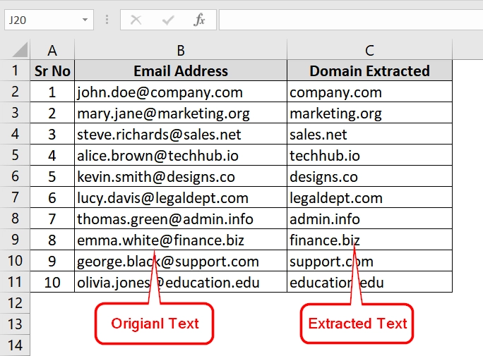
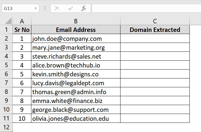
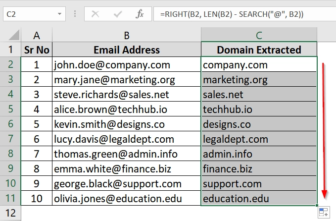
➤ Open your datasheet. We have a demo Excel worksheet with email addresses in Column B, starting from cell B2.
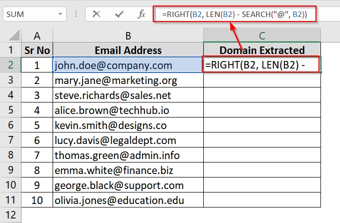
➤ Click on cell C2 where you want to extract the domain (text after “@”).
➤ Enter the formula in cell C2:
=RIGHT(B2, LEN(B2) – SEARCH(“@”, B2))
Here,
- SEARCH(“@”, B2) finds the position of “@”.
- LEN(B2) gets the total length of the email address.
- Subtracting the position of “@” from the total length gives the number of characters after it.
- RIGHT extracts that many characters from the right end of the string.
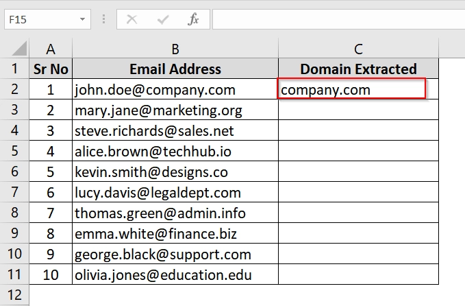
➤Press Enter. You will now see the domain name (e.g., company.com) in cell C2.
➤ Drag the fill handle down from cell C2 to apply the formula to the rest of the column for all rows.
Note:
➧ You can use FIND instead of SEARCH if you’re sure that case sensitivity won’t matter (both work similarly here).
➧ If the email address does not contain “@”, the formula will return an error. Use IFERROR for cleaner results: =IFERROR(RIGHT(B2, LEN(B2) – SEARCH(“@”, B2)), “”)
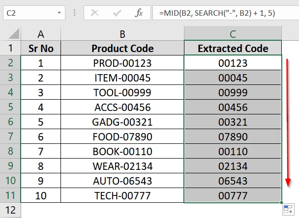
Implementing MID + SEARCH (Character-Limited Extraction)
The combination of MID and SEARCH functions allows you to extract a specific number of characters that start immediately after a defined character (such as a hyphen -). This method is useful to extract part codes, IDs, or formatted strings from structured entries.
Steps:
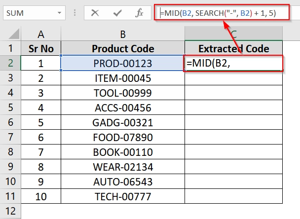
➤ Open your Excel worksheet.
➤ Enter the following formula in cell C2:
=MID(B2, SEARCH(“-“, B2) + 1, 5)
➤ Press Enter. You will now see the extracted number (e.g., 00123) in cell C2.
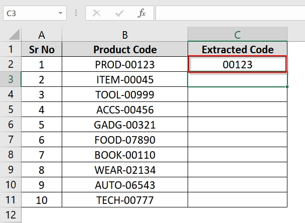
➤ Drag the fill handle down from cell C2 to fill the formula for the rest of the rows in the dataset.
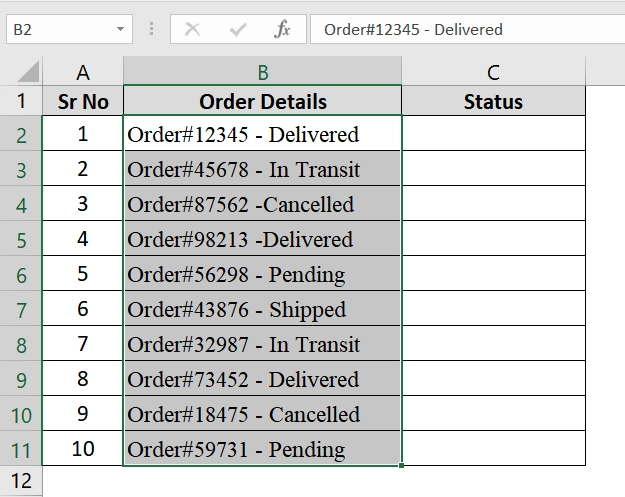
Text to Columns Feature to Perform the Split and Extract Text After a Character
The Text to Columns feature in Excel is a built-in tool that we use to split text into separate columns using a specified delimiter. It’s useful when we are working with structured text that contains characters like dashes (-), commas, or colons separating values. No formulas are required in this method.
Steps:
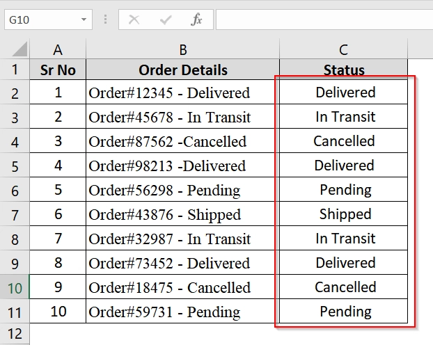
➤ Open your Excel sheet and select the range containing the text you want to split. In this example, select cells B2 to B11, which contain the “Order Details”.
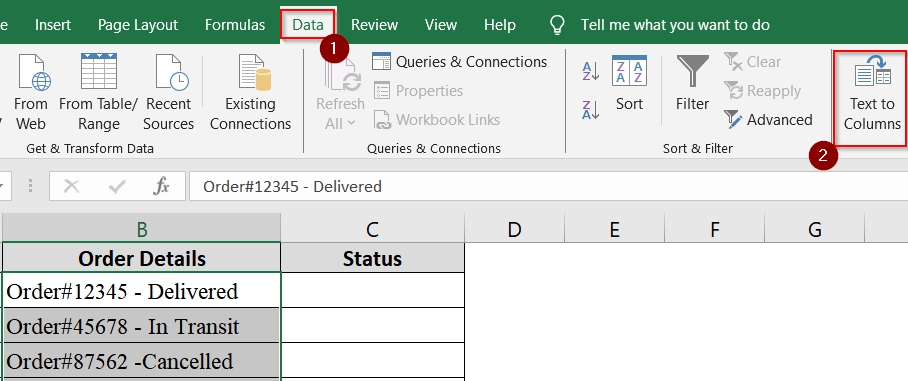
➤ Go to the Data tab on the Excel Ribbon.
➤ Click on Text to Columns in the Data Tools group.
➤ Choose Delimited in the Convert Text to Columns Wizard. Click Next.
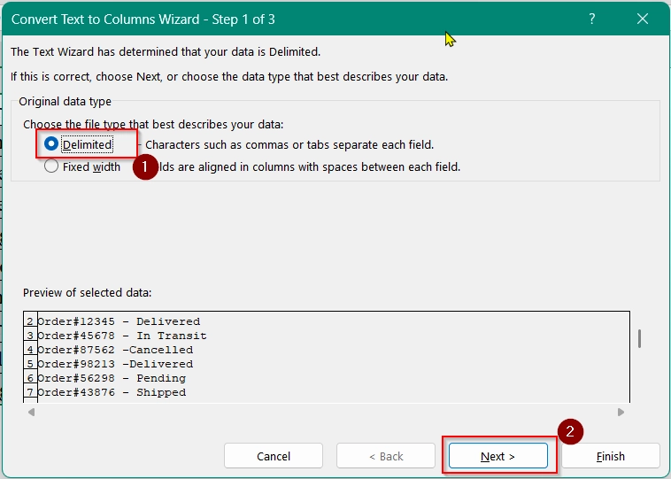
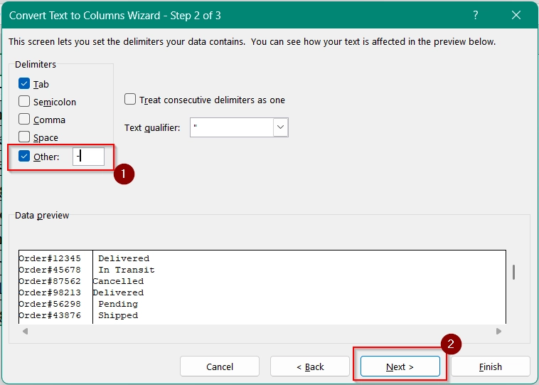
➤ In the list of delimiters, check the box for Other, and type a hyphen (-) in the box. Click Next.
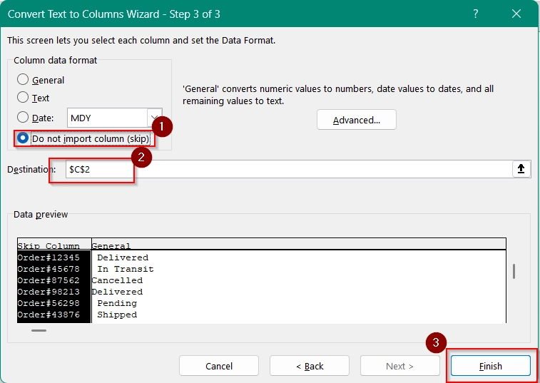
➤ Select the “Do not import column (skip)”
➤ Select the destination cell for the split text (e.g., $C$2), or let it overwrite the original column.
➤ Click Finish.
➤ Now you will see your data is extracted.
Frequently Asked Questions (FAQs)
How do I extract part of a text string in Excel?
Use the MID, LEFT, RIGHT functions along with FIND or SEARCH to specify exactly which part of the string to return.
How do you split a cell in Excel after number of characters?
Use RIGHT, LEFT, or MID with a fixed number. For example, =RIGHT(A1, LEN(A1)-5) extracts everything after the first 5 characters.
Concluding Words
We have shown some very useful and simple to use methods in this article for extracting text after a character in Excel. It’s easy once you understand the method. I have described methods for modern users to classic users with MID + FIND or even Text to Columns. Just choose the method that fits your dataset and version best and apply it.