How to Compare Two Excel Sheets for Duplicates (6 Simple Ways)

When you are working with multiple datasets in Excel, you may have repeated values in your different sheets. These duplicates in values can obviously lead to errors and confusion in reports if you don’t handle them properly.

However, it is not a very difficult task. That’s because Excel offers different ways to compare sheets and find duplicates easily. In this article, we’ll show how you can compare two sheets for duplicates using five different methods. They include visual comparison, applying formulas, Conditional Formatting, using VBA script, and Power Query.

What Does It Mean to Compare Two Excel Sheets for Duplicates?

To put it simply, you want to check both Excel sheets to find which values or records appear in both by comparing the two sheets for duplicates. So, basically, you are identifying repeated data from those two sheets. It is useful for cleaning up data, merging lists, verifying records, or avoiding errors due to duplicate entries.

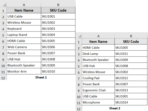
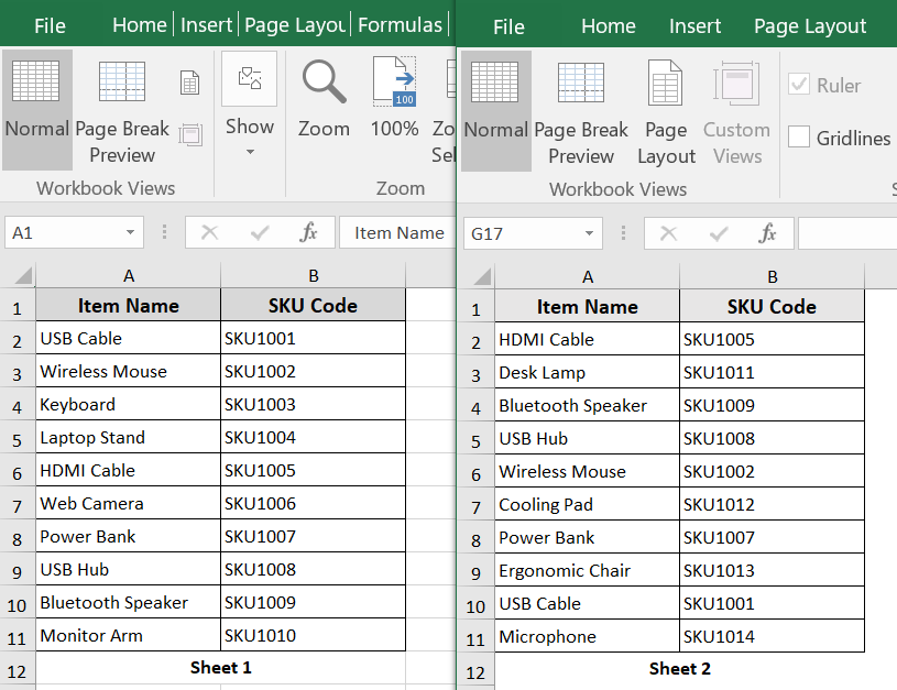
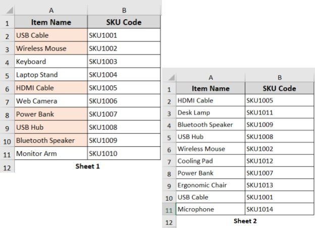
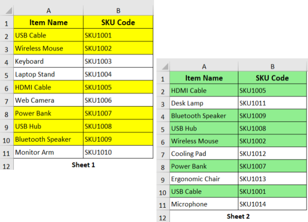
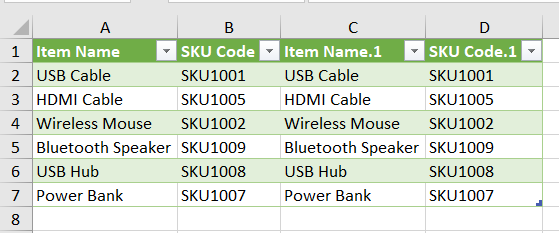
Below we have a product inventory dataset in two Excel sheets, Sheet1 and Sheet2. Here, the sheets include item names and their SKU code. Some of these entries appear in both sheets. We will now compare these two Excel sheets for duplicates using five different methods.

If you have relatively small Excel sheets and prefer to manually compare side by side, it can be a quick and easy way. The Excel built-in View tool lets you arrange two Excel windows side by side. You can use this method to visually compare two Excel sheets.

Steps:

➤ Open the Excel file that contains both Sheet1 and Sheet2.
➤ Go to the View tab >> New Window. It will open a second view of the same workbook.
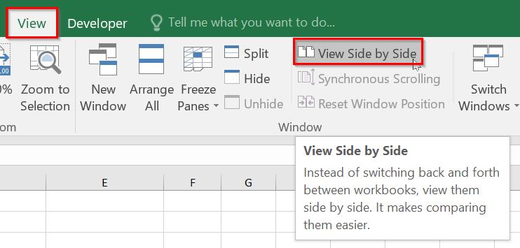
➤ In the View tab, click View Side by Side.

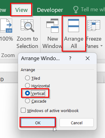
➤ By default, it will display two Excel windows horizontally. Go to View >> Arrange All >> choose Vertical >> click OK.

➤ Two separate Excel windows will be arranged side by side. Go to Sheet1 in Window1 and Sheet2 in Window2.

You can also use formulas to compare two Excel sheets and find duplicates. Excel formulas can be an easy way when you are looking to find duplicates a bit more precisely.

COUNTIF Function

The COUNTIF function checks how many times the value of Sheet1 has appeared within the range of Sheet2. When it is a match, the function returns a number 0 or greater than 0.

Steps:

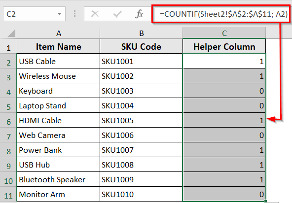
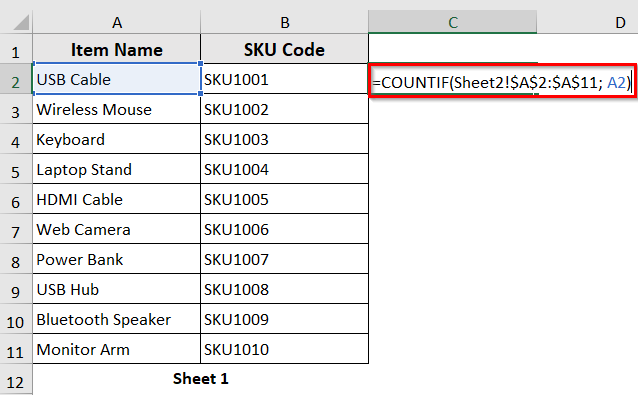
➤ Insert the below formula in the C2 cell of the helper column in Sheet1.

➤ Press Enter and use autofill
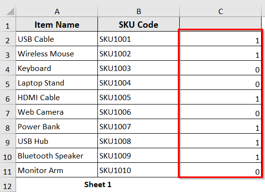
➤ The helper column shows the number of times the value of Sheet1 has appeared in Sheet2.

VLOOKUP with IF Function

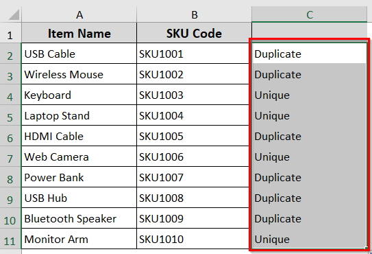
This method combines the VLOOKUP() and IF() functions. It looks for the value in Sheet1 within the range of Sheet2. If found, it returns “Duplicate.” Otherwise, it returns to “Unique.”

Steps:

➤ In Sheet1, add a helper column next to your data. ‘
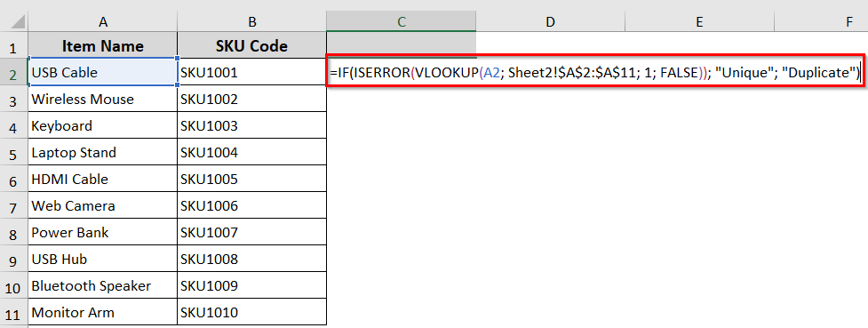
➤ Enter the following formula in the C2 cell of the helper column.

➤ Press Enter >> Use Autofill to apply the formula in the entire column.
➤ It will label each row as Duplicate or Unique based on Sheet2.

Combination of SUMPRODUCT and EXACT Functions

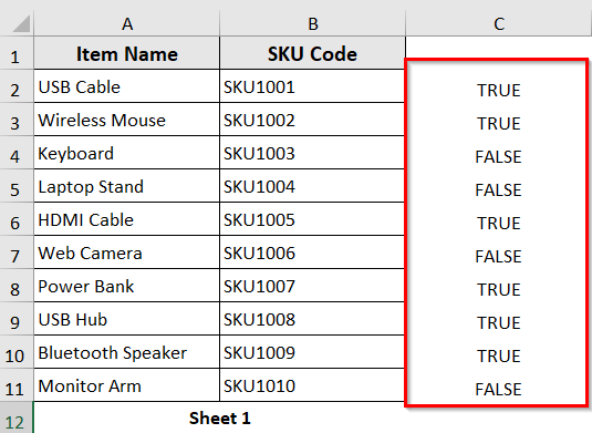
SUMPRODUCT combined with the EXACT function checks for matches between Sheet1 and Sheet2. The function returns TRUE for duplicates and FALSE for unique values.

Steps:

➤ Enter the following formula in the C2 cell.

➤ The formula will label the rows as TRUE and FALSE. TRUE means the match exists, and FALSE means the value is unique.

Conditional formatting is a quick and visual way to identify duplicate values between two sheets. It is a suitable method for simple comparisons when you’re working with small Excel data sets.

Steps:

➤ In Sheet1, select the column or range you want to compare.
➤ Go to Home tab >> Conditional Formatting >> New Rule…

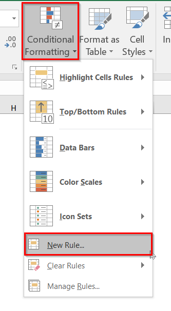
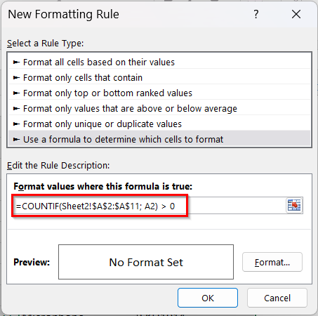
➤ Select “Use a formula to determine which cells to format”.

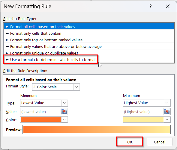
➤ Enter the following formula

➤ Click Format… >> choose Fill color >> click OK.

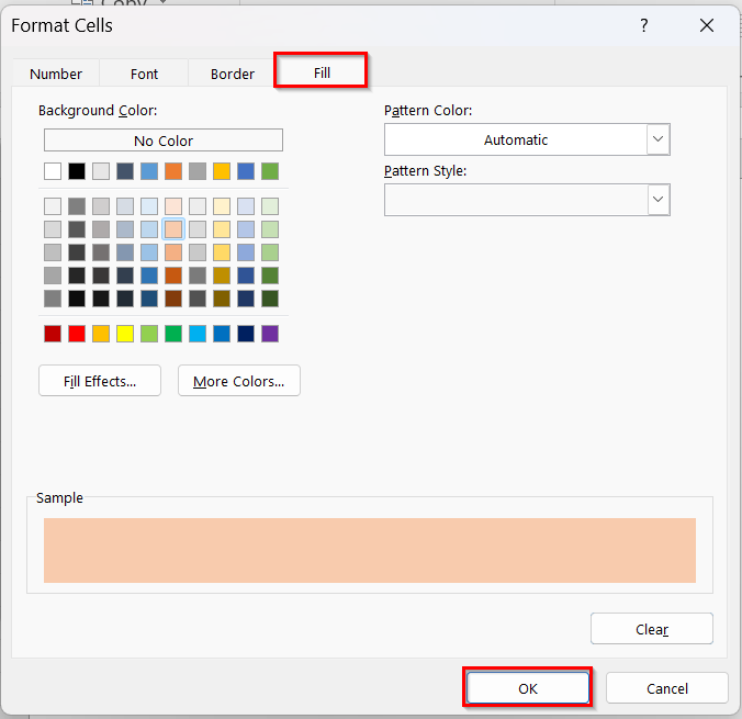
➤ Click OK again to apply the rule.
➤ The formula will highlight any duplicate values from Sheet2 in Sheet1.

If you have to compare Excel sheets regularly, VBA macros can automate the process for you. You can quickly find the duplicates between two sheets and highlight them. The process saves you time and effort.

Steps:

➤ Press  Alt  +  F11  to open the VBA editor.
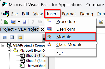
➤ Click Insert >> Module.

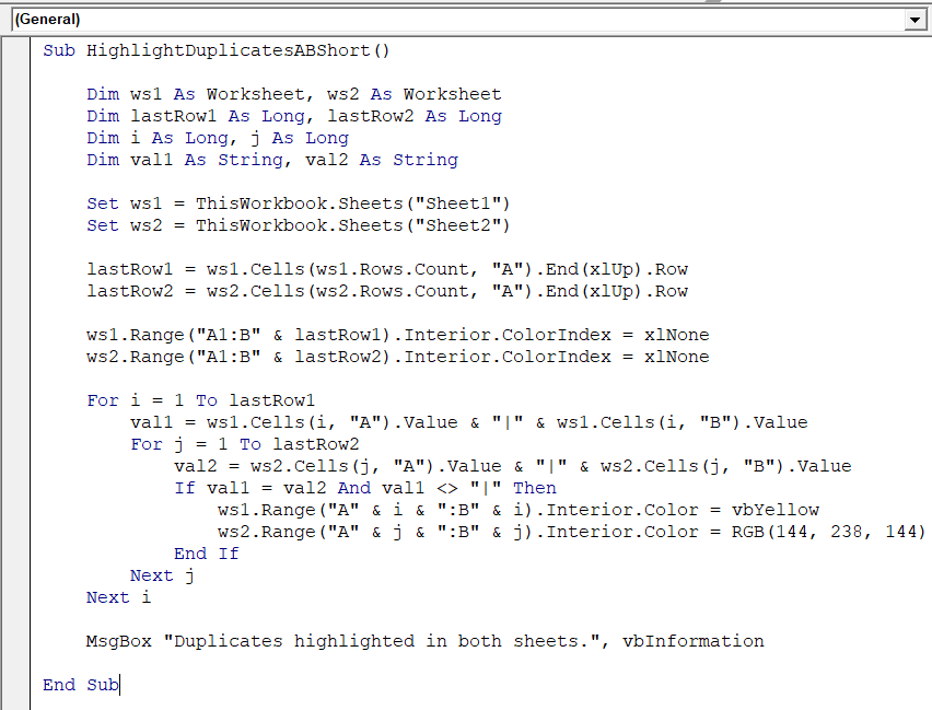
➤ Insert the below VBA script in the module.

Sub HighlightDuplicatesABShort()
    Dim ws1 As Worksheet, ws2 As Worksheet
    Dim lastRow1 As Long, lastRow2 As Long
    Dim i As Long, j As Long
    Dim val1 As String, val2 As String
    Set ws1 = ThisWorkbook.Sheets("Sheet1")
    Set ws2 = ThisWorkbook.Sheets("Sheet2")
    lastRow1 = ws1.Cells(ws1.Rows.Count, "A").End(xlUp).Row
    lastRow2 = ws2.Cells(ws2.Rows.Count, "A").End(xlUp).Row
    ws1.Range("A1:B" & lastRow1).Interior.ColorIndex = xlNone
    ws2.Range("A1:B" & lastRow2).Interior.ColorIndex = xlNone
    For i = 1 To lastRow1
        val1 = ws1.Cells(i, "A").Value & "|" & ws1.Cells(i, "B").Value
        For j = 1 To lastRow2
            val2 = ws2.Cells(j, "A").Value & "|" & ws2.Cells(j, "B").Value
            If val1 = val2 And val1 <> "|" Then
                ws1.Range("A" & i & ":B" & i).Interior.Color = vbYellow
                ws2.Range("A" & j & ":B" & j).Interior.Color = RGB(144, 238, 144)
            End If
        Next j
    Next i
    MsgBox "Duplicates highlighted in both sheets.", vbInformation
End Sub

➤ Press  F5  or click Run.
➤ It will show the following message >> Click OK.

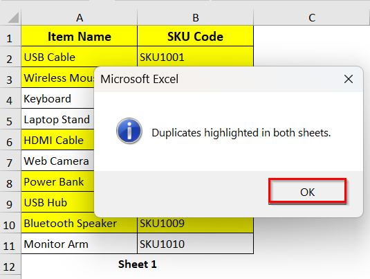
➤ The VBA script will highlight the duplicates in both sheets.

When you are working with large datasets, you can use Power Query to quickly compare two sheets and find duplicates. It will help you to find the matching values of selected columns of two sheets with accuracy. It shows results in another sheet. So, your original data remains untouched.

Steps:

➤ Click any cell in Sheet1.
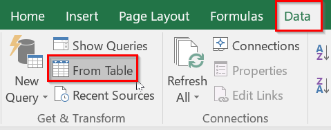
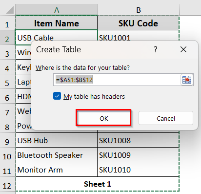
➤ Go to Data tab >> From Table

➤ It will automatically detect your table range. Ensure ‘My Table has headers’ is checked.
➤ Click OK.

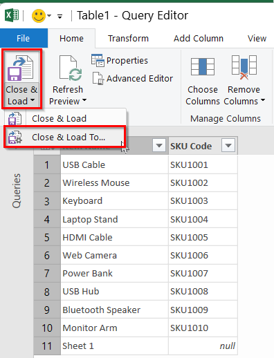
➤ When the Power Query editor opens, click Close & Load >> Close & Lead To…

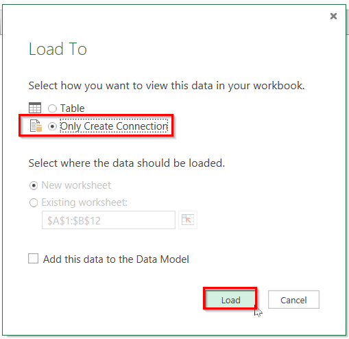
➤ Then select ‘Only Create Connection’ >> Load
➤ Repeat the same process with Sheet2.

➤ It will load both tables in the Power Query editor.
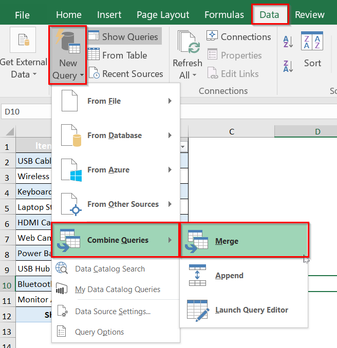
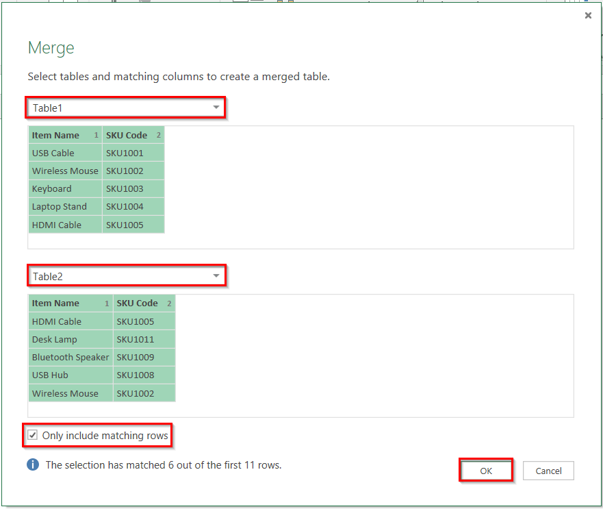
➤ In Excel, go to Data >> New Query >> Combine Queries >> Merge.

➤ In the Merge table, select Sheet1 as Table1 and Sheet2 for Table2.
➤ Check ‘Only include matching rows’ >> click OK.

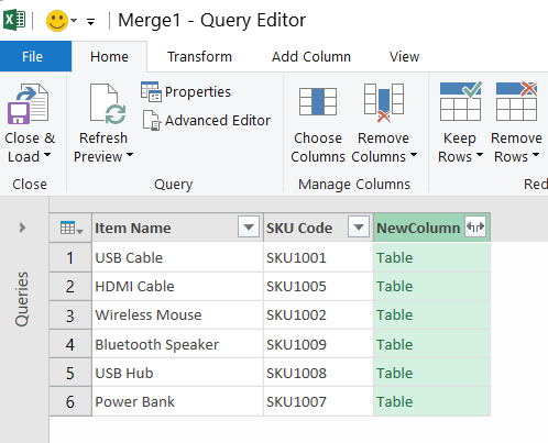
➤ After merging, you’ll see a new column next to your table with an expand icon.

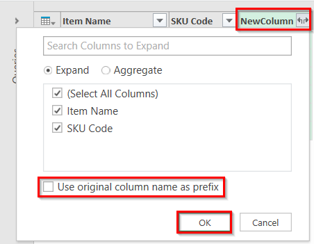
➤ Click on the expand icon >> Select the columns you want to include from Table2 >> Uncheck ‘Use original column name as prefix’ >> click OK.

➤ Select Close & Load.

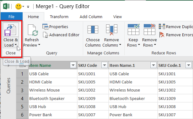
➤ Your comparison results will appear in the new sheet.

Frequently Asked Questions

How do you automatically compare two Excel spreadsheets for differences?

You can use Excel’s built-in Spreadsheet Comparison tool to compare two Excel spreadsheets automatically. The steps are below:
➤ Go to Data tab >> Data Tools >> Spreadsheet Compare
➤ Choose Compare Files >> Select two Excel files you want to compare
➤ Choose the desired comparison options >> click OK.

How to compare two columns of data in Excel?

You can use the IF function to compare two columns of data in Excel. For example, if your two columns contain car brand data, use the below IF formula:
=IF(A2=B2, “Same car brands,” “Different car brands”)
The formula will return to “Same car brands” for every TRUE value.

How to use the MATCH function in Excel?

You can use the MATCH function to find the position of a value in a list or range. Here is the syntax:
MATCH(lookup_value, lookup_array, [match_type])
➝ lookup_value: what you are looking for.
➝ lookup_array: where you are looking
➝ match_type: 0 for exact match.

Wrapping Up

In this quick tutorial, we have covered five easy ways to compare two Excel sheets for duplicates. You can apply these techniques to clean and manage your data efficiently. Download the sample Excel sheet to practice, and let us know how it has enhanced your productivity.