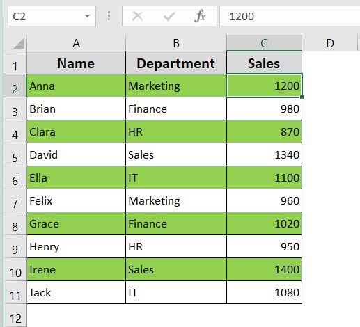
When working with large datasets, it can be difficult to read data across rows without visual guides. Alternating row colors, often called “zebra striping,” improves readability by adding subtle background shading to every other row. While Excel Tables can do this automatically, many users prefer not to convert their data into Table format.
In this article, you’ll learn how to alternate row colors in Excel without using a Table, using Conditional Formatting and formulas. This gives you full control over your data formatting while keeping things lightweight and customizable.
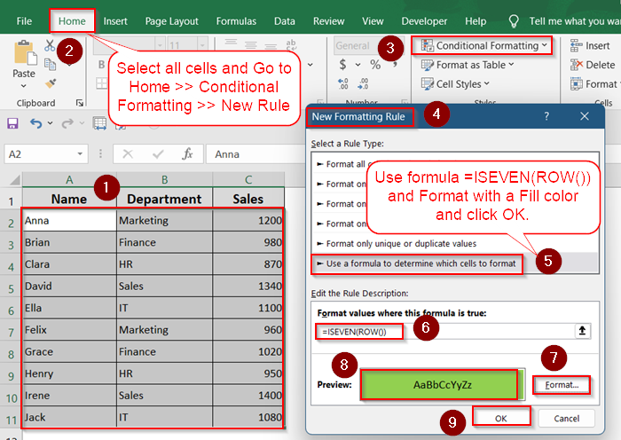
➤ Select all cells.
➤ Go to Home >> Conditional Formatting >> New Rule >> Use a formula.
➤ Type this formula: =ISEVEN(ROW())
➤ Choose a Fill color from Format.
➤ Click OK.
Use Conditional Formatting with ISEVEN Formula
This is the most popular method to apply zebra striping to rows without converting the range into a Table. It uses the ISEVEN function inside Conditional Formatting to check row numbers and apply color formatting accordingly.
This approach is quick, doesn’t require advanced formulas, and works across Excel 2010, 2013, 2016, 2019, and Excel 365.
Steps:
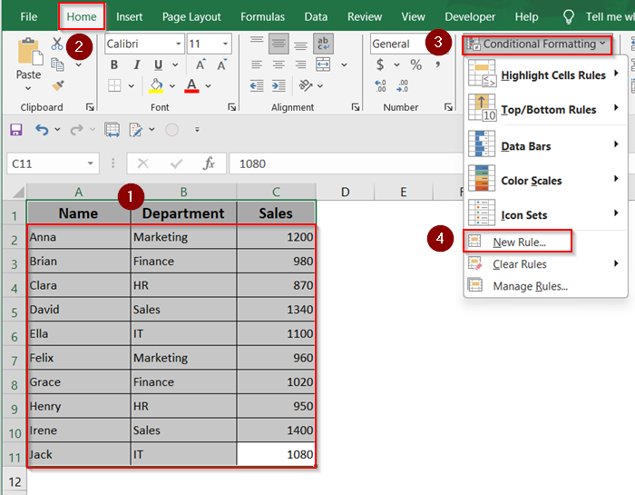
➤ Select the range you want to format (e.g., A2:C11).
➤ Go to the Home tab >> click Conditional Formatting >> choose New Rule.

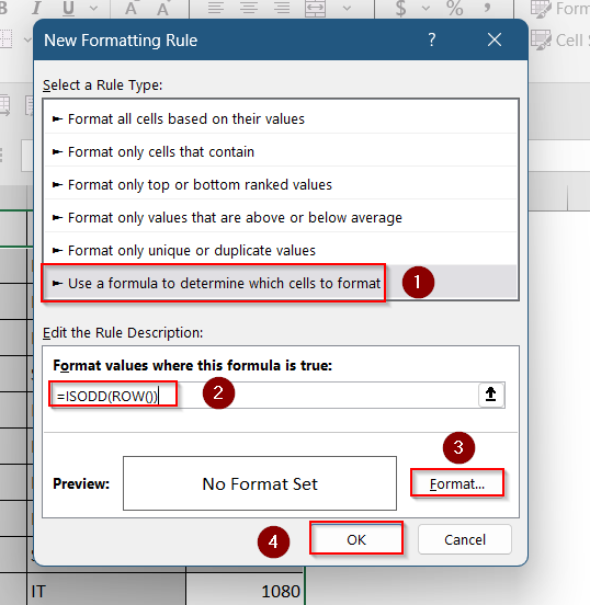
➤ Choose “Use a formula to determine which cells to format”.
➤ Enter this formula:
=ISEVEN(ROW())
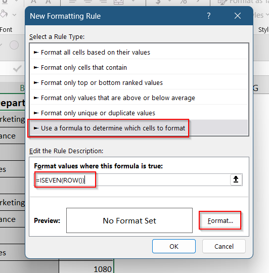
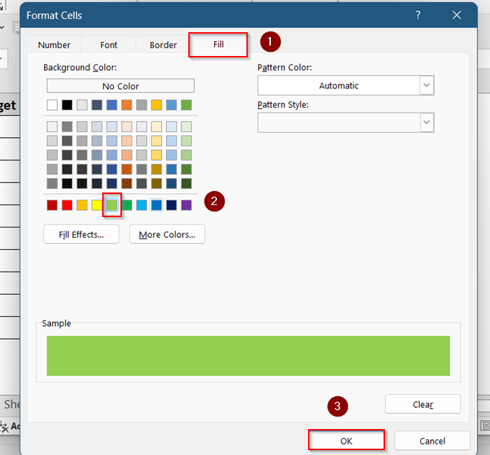
➤ Click Format, go to the Fill tab, and choose your background color.

➤ Press OK twice.
Now every even-numbered row in your range will be shaded automatically.

Choose MOD Function Instead of ISEVEN
If you want a bit more flexibility or compatibility with older versions of Excel, you can use the MOD function to achieve the same result. MOD checks if the remainder of a division operation is zero, ideal for detecting even/odd rows.
This method is useful if you prefer not to rely on ISEVEN/ISODD functions or need to fine-tune row patterns.
Steps:
➤ Select your target range (e.g., A2:C11).
➤ Go to Home >> Conditional Formatting >> New Rule.
➤ Select “Use a formula to determine which cells to format.”
➤ Enter the following formula:
=MOD(ROW(),2)=0
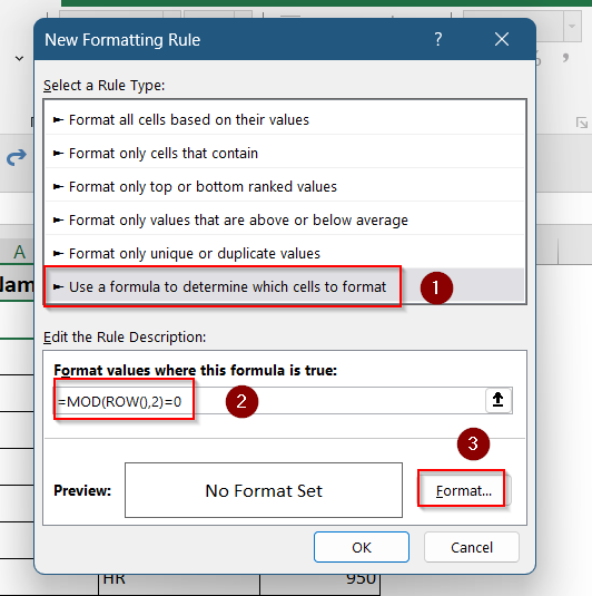
➤ Click Format, pick a fill color under the Fill tab, and hit OK.

➤ Hit OK again to apply it.
You’ll now see alternate shading on even-numbered rows across your selected area.
Apply Shading to Odd Rows Instead
By default, the above methods apply color to even rows. But if you want to start with shading on the first data row (Row 2), you can adjust the formula to highlight odd rows instead.
This is useful if your dataset begins immediately after the header row and you want your first data row shaded.
Steps:
➤ Select your range (e.g., A2:C11).
➤ Go to Home >> Conditional Formatting >> New Rule.

➤ Use this formula instead:
=ISODD(ROW())
➤ Format it with a fill color of your choice.
➤ Confirm by clicking OK.
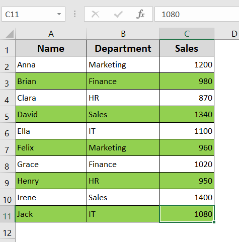
Now the odd-numbered rows in your range are highlighted, starting from Row 2.
Highlight Every Nth Row
Want to shade every 3rd or 4th row instead of every other row? You can modify the formula using MOD to create custom striping patterns.
This is especially helpful for grouped data or datasets that need visual separation every few rows.
Steps:
➤ Select the range (e.g., A2:C11).
➤ Go to Home >> Conditional Formatting >> New Rule.

➤ Use formula:
=MOD(ROW(),3)=0
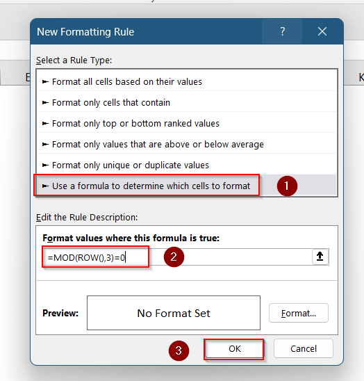
➤ Set a background fill in the Format options.

➤ Apply the rule by clicking OK.
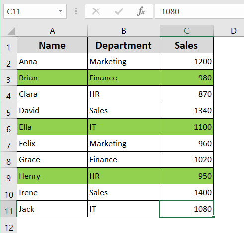
Now Excel will shade every 3rd row in your range. You can change 3 to any number to customize your pattern.
Frequently Asked Questions
Can I alternate row colors across the whole sheet?
Yes. Press Ctrl + A to select the entire worksheet, then apply Conditional Formatting using a formula like =ISEVEN(ROW()). This highlights every alternate row, keeping the full sheet striped automatically.
What happens if I insert or delete rows?
Excel automatically adjusts Conditional Formatting when you insert or delete rows. The even-odd row pattern remains intact, so your alternate row colors stay consistent without needing to manually fix anything.
Can I use different colors for even and odd rows?
Yes, you can set up two separate Conditional Formatting rules, one for even rows and one for odd rows. Use =ISEVEN(ROW()) and =ISODD(ROW()) with different fill colors.
Will this affect printing or exporting to PDF?
No. The alternate row colors created through Conditional Formatting are preserved when you print or export your sheet to PDF. This helps keep the visual layout clean and readable.
Wrapping Up
In this tutorial, you learned how to alternate row colors in Excel without using a Table. Whether you’re using the ISEVEN formula, MOD function, or a custom Nth-row approach, Conditional Formatting gives you powerful visual control over your data. These tricks keep your sheets clean, readable, and professional without the extra baggage of Table formatting. Feel free to download the practice file and share your thoughts and suggestions.