
When you’re dealing with large data tables in Excel, it can be helpful to visually identify the lowest value within columns or rows. Instead of scanning the data manually, it makes your large dataset easier to read and saves you time.
In Microsoft Excel, there are certain ways to highlight the lowest value with Conditional Formatting. In this article, we’ll show you two different ways to do so: one with Excel built-in rules and another with a custom formula for more flexibility.
➤ You can highlight the lowest value in Excel using built-in Conditional Formatting.
➤ You can also use a custom formula within conditional formatting for more control.
➤ Based on your specific need, you can highlight the entire row containing the lowest value in a specific column.
Highlighting the Lowest Value Using Built-in Rules
In simple words, highlighting the lowest value means using Excel, you want to automatically find out and mark the smallest value in a range of cells. The method makes your data analysis process easier.
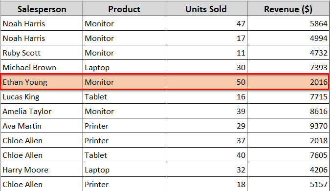
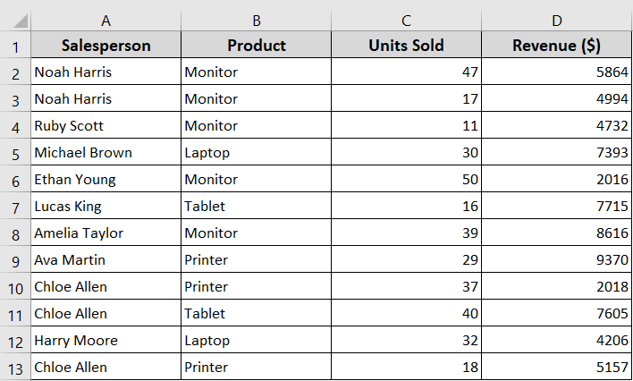
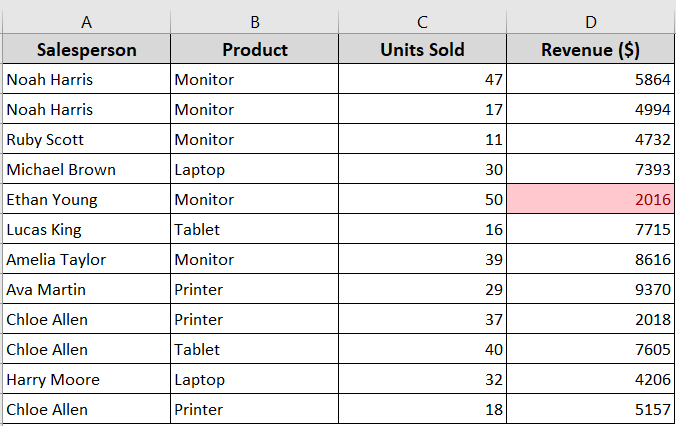
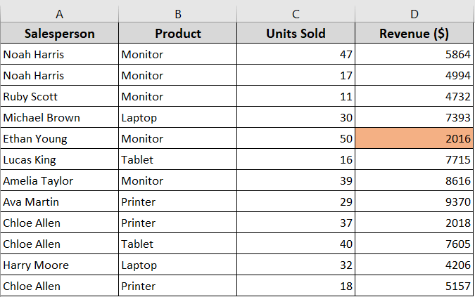
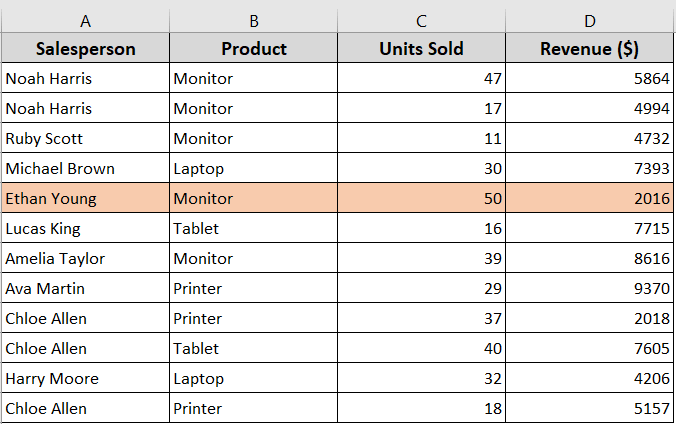
In the following dataset, we’ve a list of sales records, including units sold and total revenue. We’re going to highlight the lowest revenue ($) value using the Conditional Formatting feature of Excel.
In this method, Excel uses the built-in rules to highlight the lowest value. It doesn’t require any formula. So, you can quickly highlight the minimum value in an Excel dataset.
Steps:
➤ Select the cells in the Revenue column.
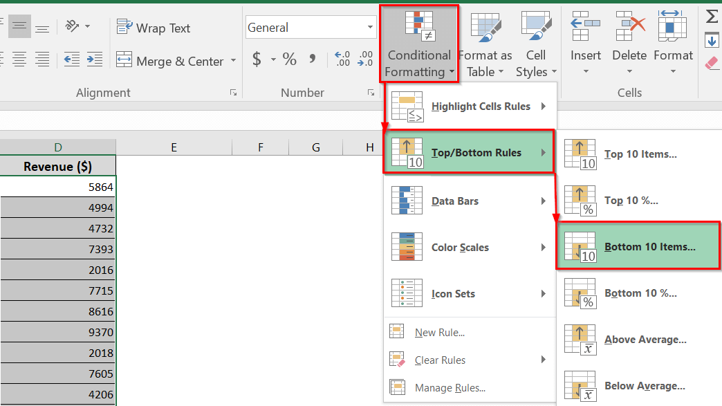
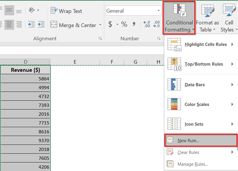
➤ On the Home tab, in the Styles group,
Click Conditional Formatting >> Top/Bottom Rules >> Bottom 10 Items…
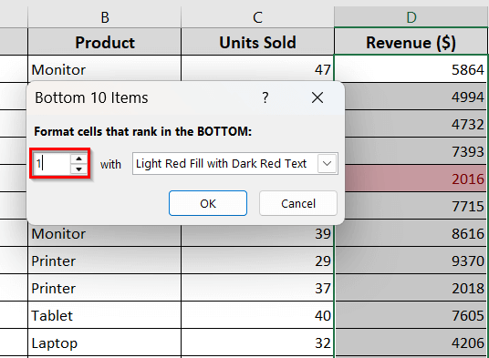
➤ A small dialog box will appear. In the dialog box, replace 10 with 1 as we’re highlighting the lowest value.
➤ Choose a formatting style that suits you. Here, we’ve used the default formatting style, Light Red Fill with Dark Red Text.
➤ Click OK.
➤ Excel will now highlight the lowest revenue value (2016) in your selected range.
Using a Custom Formula to Highlight the Lowest Value
When you use a custom formula within Conditional Formatting, it gives you more control over what gets highlighted and flexibility in your highlighting rules. You can use the method to highlight the lowest value based on a specific criterion.
Steps:
➤ Click and drag to select the range you’d like to highlight numbers.
➤ In the Home tab, select Conditional Formatting >> New Rule…
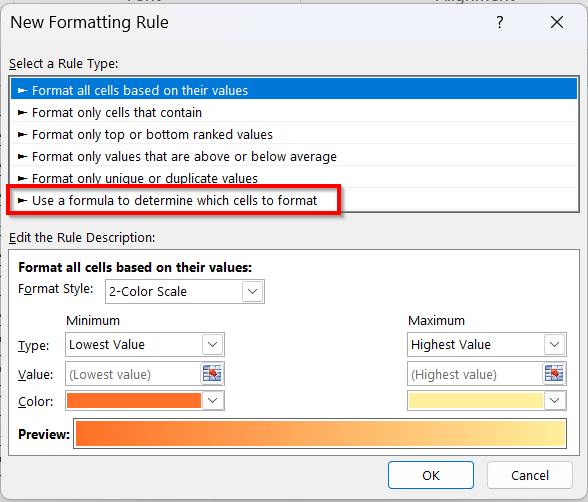
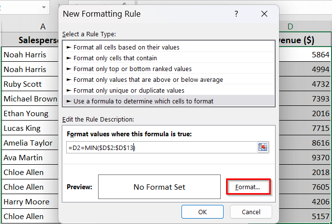
➤ Select “Use a formula to determine which cells to format” in the New Formatting Rule dialog.
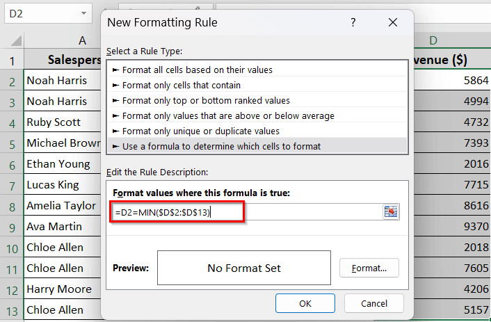
➤ In the formula box, enter the following custom formula:
=D2=MIN($D$2:$D$13)
➥ $D$2:$D$13: Full range of cells where you’re checking for the lowest value. The $ sign means the range remains fixed.
➥ MIN($D$2:$D$13): It finds the smallest number in your chosen range.
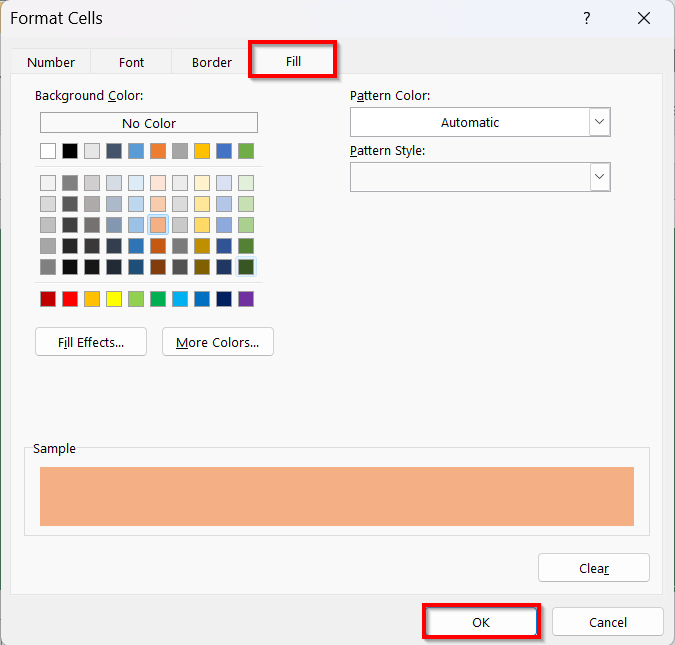
➤ Click the Format >> Fill option.
➤ Choose a fill color to highlight the cell.
➤ Click OK.
➤ Click OK again, and Excel will highlight the lowest value in your selected range.
Highlighting the Entire Row Based on the Lowest Value
This method highlights the entire row where the lowest value appears in the selected cells. It is helpful when you want to track the full record, not just one cell.
Steps:
➤ In this case, select the full table range without the header row.
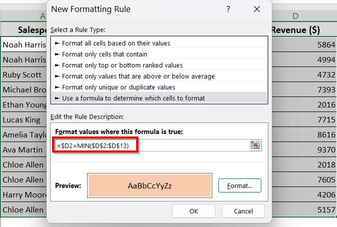
➤ Go Home tab >> Conditional Formatting >> New Rule >> Choose Use a formula to determine which cells to format.
➤ In the formula box, enter the following formula:
=$D2=MIN($D$2:$D$13)
➥ MIN($D$2:$D$13): It finds the lowest revenue in your range.
➤ Choose the formatting style. Click OK.
➤ Click OK again to apply the rule.
➤ Excel will now automatically highlight the entire row where the lowest revenue appears.
Frequently Asked Questions
How do you find the lowest value in Excel with multiple criteria?
You can use the syntax of MINIFS to find the lowest value with multiple criteria in Excel. Use the following formula
=MINIFS(D2:D15, A2:A15, F2, C2:C15, F3)
Here,
- D2:D15: The range of cells where Excel looks for the minimum value
- A2:A15: First criteria range
- F2: First condition
- C2:C15: Second criteria range
- F3: Second condition
Excel will check both conditions and find out the lowest value from the selected rows.
How to select the lowest value in Excel?
The MIN function can help you find the lowest value in Excel. It scans the selected range and returns the smallest number.
The formula is below:
=MIN(A2:A7).
This formula will check all the values from cell A2 to cell A7 and return the lowest value among them.
How do you find the lowest to highest in Excel?
Follow the steps below to find the lowest to highest in Excel using the SORT feature.
➤ Select your data range.
➤ Click a cell in the column you want to sort by.
➤ Go to the Data tab >> Sort & Filter group >> Sort A to Z.
➤ It will sort your data from lowest to highest order.
What is the formula for the lowest common multiple in Excel?
You can use the LCM formula to find out the lowest common multiple in Excel. We use the formula, =LCM(number1,[number2],…) to calculate LCM. Here, number 1 and number 2 are the integers you want to find the LCM of.
Wrapping Up
In today’s quick guide, we’ve learned two simple ways to highlight the lowest value in Excel using Conditional Formatting. Both methods help you find out the lowest data points faster with less effort. Feel free to try out the sample Excel sheet we’ve used for practice, and let us know how these techniques have enhanced your data analysis.