only the largest/first or smallest/last occurrence of a match, you need a formula with the MAX or SMALL function. With the MAX function, Excel returns the largest value from a set of n
To apply various Excel rules, such as data validation, conditional formatting, and dynamic charts, knowing the row number of certain values or cells can be essential. For complex datasets, using a formula is a straightforward and dynamic solution to return the row number of a cell or value match.
Therefore, we’ll apply the ROW, IF, and MIN functions to determine which row number in the sheet has the first occurrence of a specific value in a defined range.
Steps to return row number of a matched data with MIN and IF functions:
➤ Select a cell to enter the input, the returned row number, and enter the following formula:
=MIN(IF(A1:D10=”Math”, ROW(A1:D10)))
➤ Here, Math is the value to match within the A1:D10 range. Change them according to your dataset.
➤ Press Enter for Excel 365/2021 and use CTRL + SHIFT + ENTER for Excel 2019 or older versions.

Other methods for finding the row number of a match include combining various Excel functions, such as ROW, MATCH, INDEX, and TEXTJOIN, and utilizing VBA coding. This article covers all the easy ways to return a row number.
Using the ROW Function to Return Row Number for a Specific Cell
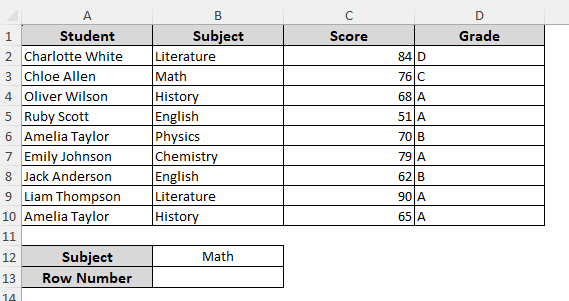
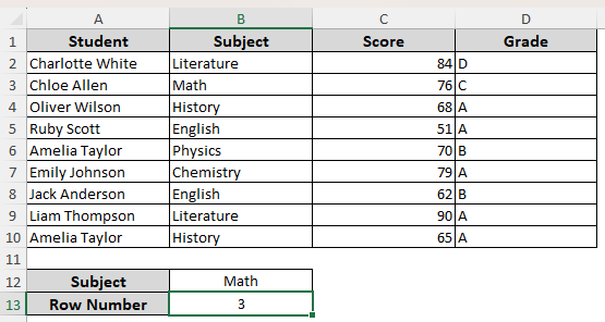
In our practice dataset, we have columns for student names and their obtained marks in different subjects. We’ll look for the value Math in column B. You can also insert the value in a different cell and use the cell reference to find a match.
As you can see, we have it in cell B3. Therefore, our formulas should return 3 as the row number. We put the value Math in cell B12. As we apply the formulas, we get the returned row number in cell B13.
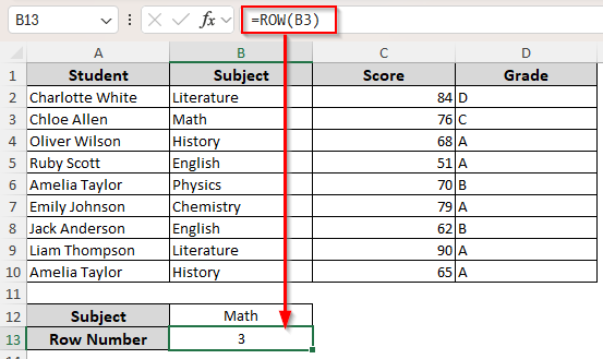
Excel’s ROW function returns the row number of a cell or range. However, it doesn’t take strings or values as references. Therefore, you need to know exactly which cell features the value you’re looking for. Here’s how it works:
➤ Select a cell where you want the returned row number. Type the following formula with the correct cell reference containing the value you want to match instead of B3 and click Enter:
=ROW(B3)
Finding Relative Row Number for a Matched Cell with the MATCH Function
While the MATCH function is ideal for looking up a value, you must know the column name carrying the value. Also, if you search for a value within a range, it returns the relative position of the row.
Therefore, we’ll use the entire column as our range to get the absolute row number. Here are the details:
➤ To find a match within a range, type the following formula and press Enter:
=MATCH(“Math”, B1:B10, 0)
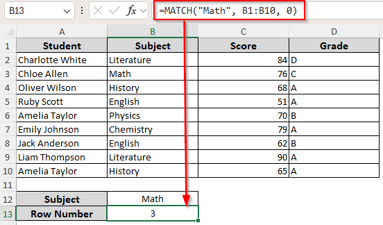
As we’ve included the first cell of the column, this formula returns the correct row number.
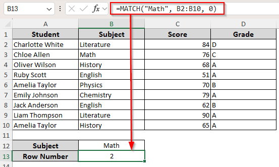
However, to get a relative row number based on the row range you select, enter the following formula:
=MATCH(“Math”, B2:B10, 0)
➤ This returns the relative position of the value, which is 2 in this case. Change the cell range as needed.
Finding Absolute Row Number for a Matched Cell/Range/Value
To always get the absolute row number, combine the MATCH and ROW functions. While the MATCH function returns the relative position in the range, the ROW function counts the first row number in the range. As we combine the two functions and subtract 1, we get the absolute row number for a selected range. Below are the steps:
➤ In the cell where you want the row number, insert any of the following formulas:
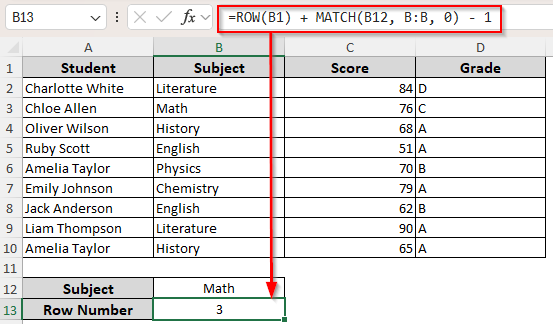
To Match A Cell Reference to An Entire Column
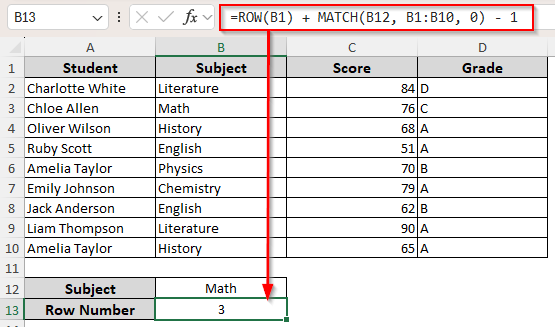
➤ First, enter the value you’re looking for in an empty cell (B12), and type this formula in a different cell(B13):
=ROW(B1) + MATCH(B12, B:B, 0) – 1
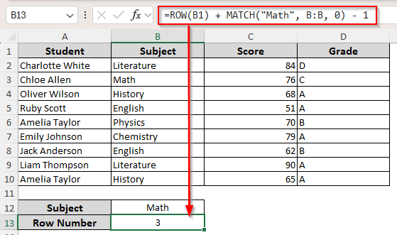
To Match A Value to An Entire Column
Enter the following formula in the output cell:
=ROW(B1) + MATCH(“Math”, B:B, 0) – 1
To Match Specific Range
Enter the following formula in the output cell:
=ROW(B1) + MATCH(B12, B1:B10, 0) – 1
➤ For each formula, you can change the value, cell reference, and column range as needed. Press Enter.
Return Row Number for a Match or Text for No Match
All the above-mentioned formulas return the #N/A error if the value isn’t matched with any cell of a column or range. If you want the formula to return texts like No Match or Match Not Found, you need to add the IFERROR and INDEX functions. While the INDEX function returns a value from a specified column, IFERROR handles errors with custom messages. Use them following the steps given below:
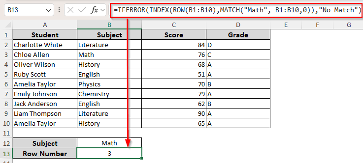
➤ Select a cell to put the row number and enter the following formula:
=IFERROR(INDEX(ROW(B1:B10),MATCH(“Math”, B1:B10,0)),”No Match”)
➤ Change the cell references and values to match based on your dataset. You can also search for a match from the entire column or a cell.
➤ Finally, click Enter.
Look for a Match and Get Row Number Across Multiple Columns and Rows
All the formulas mentioned above work on a single column at a time. Therefore, you need to know which column contains the value you’re looking for.
Otherwise, you have to repeat the process for each column. To avoid this and find a match across all the columns and rows, we’ll combine the IF, ROW, and MIN functions.
The IF function checks the cells for a defined value and returns an array of row numbers. Whereas, the MIN function returns the smallest value within an array. Here’s how to use them:
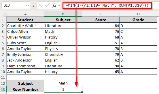
➤ Pick a cell to get the returned row number and enter the following formula:
=MIN(IF(A1:D10=”Math”, ROW(A1:D10)))
➤ Instead of Math, you can enter a cell reference containing the value you’re looking for. Replace the cell range as required.
➤ Click Enter for Excel 365/2021 or newer versions. For Excel 2019 or older versions, press CTRL + SHIFT + ENTER .
Return Several Row Numbers for Multiple Matches
If the value you’re looking for occurs in multiple rows, the previous functions might not return the ideal match. Therefore, to get all the row numbers and separate them with a defined delimiter, we’ll combine the TEXTJOIN function with IF and ROW.
The TEXTJOIN function combines multiple results from various ranges/strings and joins them in a single string. Here, we’ll join the row numbers with a comma (,). Let’s get to the steps:
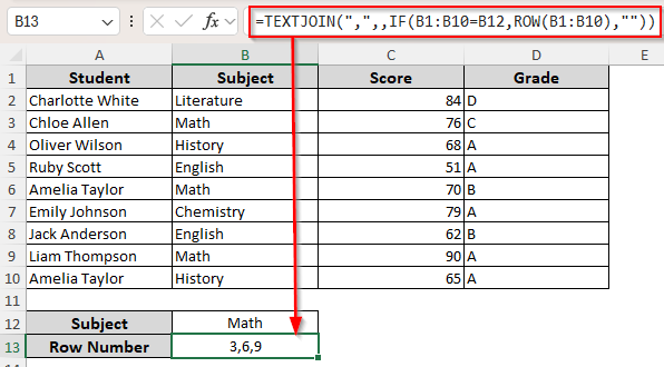
➤ In your preferred blank cell, enter the following formula:
=TEXTJOIN(“,”,,IF(B1:B10=B12,ROW(B1:B10),””))
➤ Replace the delimiter, column range, and cell reference containing the value according to your dataset.
➤ Click Enter for new Excel versions and CTRL + SHIFT + ENTER for the old ones (before 2019).
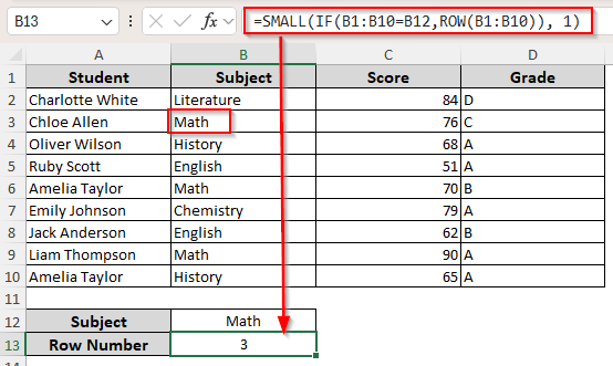
Return the First or Last Row Number for Multiple Matches
When you want only the largest/first or smallest/last occurrence of a match, you need a formula with the MAX or SMALL function. With the MAX function, Excel returns the largest value from a set of numbers, which will be the last occurrence of the value.
The SMALL function returns the smallest one, which is the first row number. Here are the steps:
➤ Choose a blank cell for the result and insert any of the following formulas:
For the Smallest/First Row Number
Enter the following formula in the output cell:
=SMALL(IF(B1:B10=B12, ROW(B1:B10)), 1)
➤ Click Enter or CTRL + SHIFT + ENTER based on the Excel version you’re using.
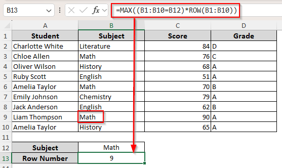
For the Largest/Last Row Number
Enter the following formula in the output cell:
=MAX((B1:B10=B12)*ROW(B1:B10))
➤ Press Enter or CTRL + SHIFT + ENTER based on the Excel version you’re using.
Return Row Number of Match with VBA Macro
In this method, we’ll utilize VBA coding to get the row number of a matched cell or value. It works across a wide range of columns and rows. You can select the range and input a value or cell reference to return the absolute row number. Below are the steps:
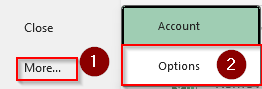
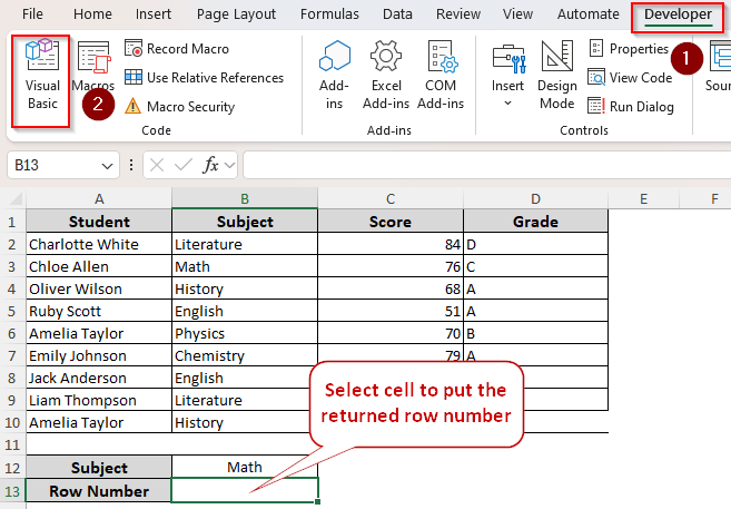
➤ Check if your main ribbon has the Developer tab. If not, go to the File tab >> More >> Options.
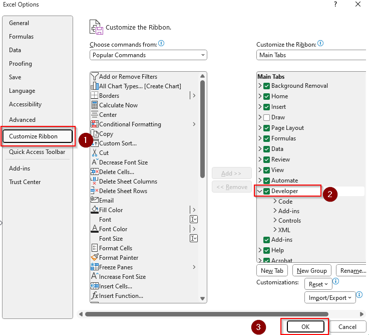
➤ Click on Customize Ribbon and check the Developer box. Press Ok.
➤ Now, select a cell to enter the returned value. Open the Developer tab and click on Visual Basic from the Code group.
➤ As the VBA Editor opens, press Insert from the tab and choose Module.
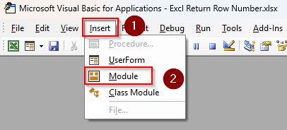
➤ Paste the following code in the Module box:
Sub FindRowNumbersOfMatch()
Dim lookupInput As String
Dim lookupValue As String
Dim searchRange As Range
Dim cell As Range
Dim resultRows As String
Dim currentCell As Range
Dim testMsg As String
' Store the cell where macro is launched
Set currentCell = Application.ActiveCell
' Get the value or cell reference to look for
lookupInput = Application.InputBox("Enter a value or cell reference to search for (e.g., A1 or John):", "Lookup Value", Type:=2)
If lookupInput = "False" Then Exit Sub ' Cancel pressed
' Attempt to interpret input as a cell reference
On Error Resume Next
Dim tempRange As Range
Set tempRange = Nothing
Set tempRange = Range(lookupInput)
On Error GoTo 0
If Not tempRange Is Nothing Then
lookupValue = Trim(CStr(tempRange.Value))
testMsg = "Interpreted input as cell reference. Value to find: '" & lookupValue & "'"
Else
lookupValue = Trim(lookupInput)
testMsg = "Interpreted input as literal value: '" & lookupValue & "'"
End If
' Ask user to select the range to search
On Error Resume Next
Set searchRange = Application.InputBox("Select the range to search in:", "Search Range", Type:=8)
On Error GoTo 0
If searchRange Is Nothing Then
MsgBox "No range selected. Exiting."
Exit Sub
End If
' Debug message showing what is searched where
MsgBox testMsg & vbNewLine & "Range selected: " & searchRange.Address
' Loop through search range to find matching rows (case-insensitive)
For Each cell In searchRange
If Not IsError(cell.Value) Then
If Len(Trim(CStr(cell.Value))) > 0 Then
If StrComp(Trim(CStr(cell.Value)), lookupValue, vbTextCompare) = 0 Then
If resultRows <> "" Then
resultRows = resultRows & ","
End If
resultRows = resultRows & cell.Row
End If
End If
End If
Next cell
' Output results to the active cell
If resultRows <> "" Then
currentCell.Value = resultRows
Else
currentCell.Value = "No match found"
End If
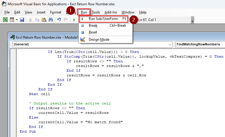
End Sub➤ Click on the Run tab and choose Run Sub/UserForm. Or, press F5 .
➤ In the Lookup Value box, enter the cell reference containing the value you’re looking for or type the value itself. Click Ok.
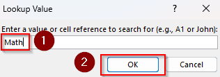
➤ As Excel prompts you to select a range to find a match, return to the Excel tab and highlight the range. Or, you can type it manually. Press Ok.
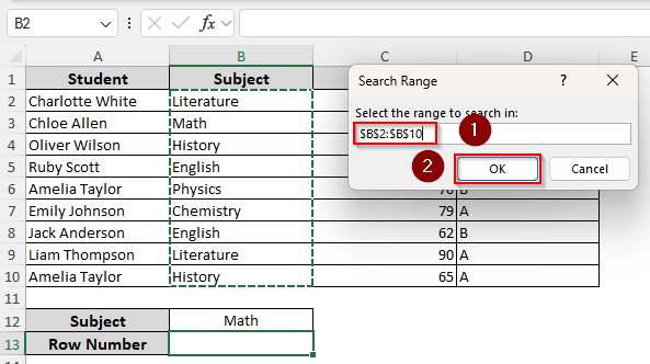
➤ Here’s the result for our dataset:
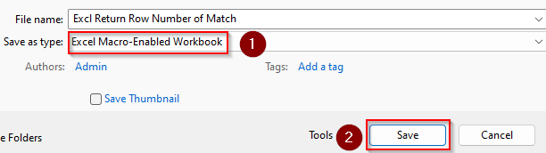
➤ To save the changes, go to the File tab and select Save As.
➤ In your desired location, click on the Save as Type box and choose Excel Macro-Enabled Workbook. Press Save.
Frequently Asked Questions
How to return the row number of the nth match?
Let’s say we’re looking for the second occurrence of the value Math. To get the row number for it, insert the following formula in a blank cell:
=SMALL(IF(B1:B10=”Math”, ROW(B1:B10)), 2)
You can change the value, range, and occurrence number as necessary. Click Enter or CTRL + SHIFT + ENTER for new or old Excel versions, respectively.
Can you return the row number of the match with XLOOKUP?
Yes, you can. The XLOOKUP function finds the first match of a cell or value. To return the row number of a match using XLOOKUP, use this formula:
=XLOOKUP(“Math”, B:B, ROW(B:B))
How do you return the row number for a partial match?
To return the row number for a partial match, such as Math for Mathematics, enter the following formula:
=MIN(IF(ISNUMBER(SEARCH(“Math”, B1:B10)), ROW(B1:B10)))
Press Enter or CTRL + SHIFT + ENTER based on your Excel version.
Concluding Words
Although several functions can return the row number for a cell or value match, they have specific uses depending on the dataset. Combining the MATCH and ROW functions is the easiest way, but it only works on one column at a time.
For a wider range, you need the formula with IF and MIN functions. To get multiple matches, use the formula with the TEXTJOIN function.