Returning all rows that match specific criteria is a common task in Excel for filtering data, creating reports, and analyzing information. Whether you want to extract sales data by region or list employees by department, Excel provides multiple ways to return full rows that meet your conditions.
In this article, you’ll learn several effective methods using functions like FILTER, INDEX, SMALL, IF, ROW, AGGREGATE, and SORT. Each technique works with different Excel versions, offering dynamic and legacy solutions for accurate and efficient data extraction.
Steps to return all rows that match criteria using the FILTER function in Excel:
➤ Select a blank cell like A13 where you want the results to appear.
➤ Enter the formula: =FILTER(A2:E11, (C2:C11=”East”)*(D2:D11>150))
➤ Press Enter to spill automatically.
Use the FILTER Function to Dynamically Extract Matching Rows
The easiest and most dynamic way to return all rows matching criteria is by using the FILTER function available in Excel 365 and Excel 2021. This function filters a range or array based on a logical test and returns all matching rows in a spill range, updating automatically when your data changes.
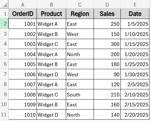
We’ll use a sample dataset containing order records with five columns: OrderID, Product, Region, Sales, and Date. It includes transactions from various regions and products, allowing us to test different filtering criteria such as finding all rows where Region is “East” and Sales exceed 150.
Steps:
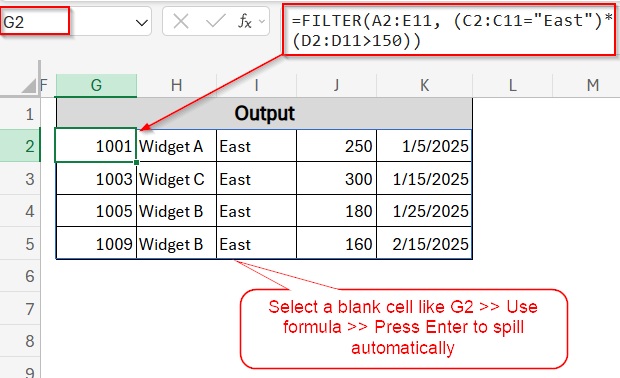
➤ Select a blank cell where you want the filtered results to appear, for example, G2.
➤ Enter the formula below to return all rows where Region is “East” and Sales are greater than 150:
=FILTER(A2:E11, (C2:C11=”East”)*(D2:D11>150))
Change A2:E11 to your full data range; update C2:C11 and D2:D11 to your filter columns and set the criteria values accordingly. If your data is on another sheet, prefix ranges with the sheet name like Sheet1!A2:E11.
➤ Press Enter and the formula will spill automatically.
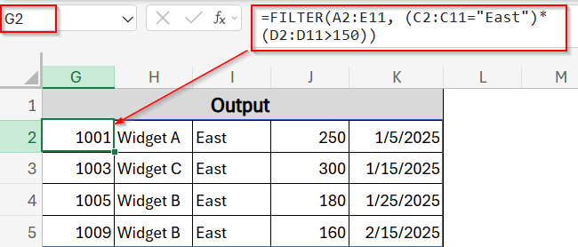
This formula checks columns C (Region) and D (Sales) for your criteria and returns every row from columns A to E that meets both conditions. The results will spill automatically below the formula, showing complete rows with all columns.
Pull Matching Rows with INDEX, SMALL & ROW Functions
If you’re working in older versions of Excel without dynamic arrays, you can still return all matching rows using this alternative formula. This method combines INDEX with SMALL and ROW to identify and extract rows that meet specific criteria. It works similarly to the previous approach but calculates row positions using ROW instead of IF.
In this case, we will test each row for “East” in column C and sales greater than 150 in column D, use ROW to collect the row numbers of matches, and SMALL to return them in ascending order. INDEX then pulls the entire matching rows from columns A to E.
Steps:
➤ Select a blank cell where you want the results to start, for example, G2.
➤ Enter the formula below, confirm with Ctrl + Shift + Enter in older Excel (just Enter in Excel 365), then drag it across five columns and down:
=IFERROR(INDEX($A$2:$E$11,SMALL(IF(($C$2:$C$11=”East”)*($D$2:$D$11>150),ROW($A$2:$A$11)-ROW($A$2)+1),ROWS($G$2:$G2)),COLUMN(A:A)),””)
Change $A$2:$E$11 to your full data range; update $C$2:$C$11 and $D$2:$D$11 to your filter columns and criteria. If the data is on another sheet, prefix ranges with its sheet name, for example, Sheet1!$A$2:$E$11.
➤ Press Enter and drag across and down as needed.
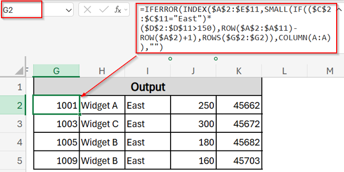
Now you have your desired output filtered by the East region and sales greater than 150.
Use IF Logic with SORT Function to Return Matching Rows Neatly
You can combine basic IF logic with Excel’s SORT and FILTER functions to return all rows that meet specific criteria and sort them for a cleaner presentation. This method is only available in Excel 365 and Excel 2021, but is extremely simple and effective for dynamic reporting.
In this case, we will filter rows where Region is “East” and Sales is greater than 150, then use SORT to arrange the returned rows in ascending order by the first column (Product). It’s a great way to display matching data in a tidy and automatically updating format.
Steps:
➤ Select a blank cell where you want the sorted, filtered results to appear, for example, G2.
➤ Enter the following formula:
=SORT(FILTER(A2:E11, (C2:C11=”East”)*(D2:D11>150)))
Change A2:E11 to your complete data range; update C2:C11 and D2:D11 to your filter columns and criteria values. If your data is in another sheet, add the sheet name before the ranges like Sheet1!A2:E11.
➤ Press Enter.
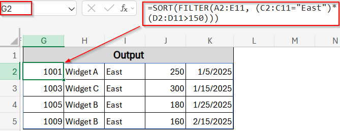
Now you have your desired output filtered by the East region and sales greater than 150.
Extract Matching Rows Using AGGREGATE with INDEX Function
The AGGREGATE function combined with INDEX offers an efficient way to return all rows that meet your criteria without requiring array formulas. It works in Excel 2010 and later versions and handles errors gracefully while calculating row positions for matching records.
The formula outputs complete rows that match both Region = “East” and Sales > 150 by using the AGGREGATE function to determine row positions. The result appears row by row and column by column, fully maintaining the structure of the original data.
Steps:
➤ Choose a blank cell where you want the filtered results to start, for example, G2.
➤ Use this formula in the selected cell:
=IFERROR(INDEX($A$2:$E$11, AGGREGATE(15, 6, (ROW($A$2:$A$11)-ROW($A$2)+1)/(($C$2:$C$11=”East”)*($D$2:$D$11>150)), ROWS($G$2:$G2)), COLUMN(A:A)), “”)
Change $A$2:$E$11 to your full data range; update $C$2:$C$11 and $D$2:$D$11 to your filter columns and criteria. If your data is on another sheet, prefix ranges with the sheet name like Sheet1!$A$2:$E$11.
➤ Press Enter, then copy the formula down and across as necessary.
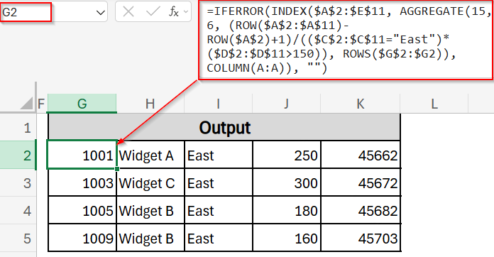
This formula is an efficient, non-array alternative for extracting matching rows displaying your filtered output in the selected cell G2.
Frequently Asked Questions
Can FILTER return all matching rows?
Yes. In Excel 365/2021, FILTER(array, criteria, “”) spills all rows that meet your conditions. It dynamically updates and automatically resizes. Just ensure your source array and criteria range align in size.
Why is FILTER missing some rows?
If FILTER isn’t showing all applicable rows, check your criteria arrays. Ensure the logical test yields TRUE for those rows, ranges are the same size, and there are no blank or error values disrupting the Boolean array.
Can VLOOKUP or XLOOKUP return multiple matching rows?
No. Both functions only return the first match. To return multiple rows, use FILTER, INDEX & SMALL, or helper columns with AGGREGATE. Functions like VLOOKUP/XLOOKUP only give a single result per lookup key.
Wrapping Up
In this tutorial, you’ve learned several effective methods to return all rows that match criteria in Excel, using formulas like FILTER, INDEX, SMALL, IF, and AGGREGATE, as well as built-in tools like the Advanced Filter. Each method has its own advantage. Some are more dynamic and modern, while others provide compatibility with older Excel versions. Feel free to download the practice file and share your feedback.