
In Microsoft Excel, we often need to merge two sheets. That can be based on one common column like a customer ID or employee number. This is useful when different pieces of information are stored across separate sheets. And when they need to be brought together for reporting or analysis. For example, you may have employee details in one sheet and salary information in another, both linked by the Employee ID.
To merge two excel sheets based on one column, follow these steps:
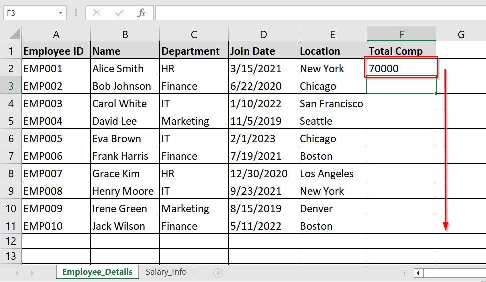
➤ Identify the common column in both Excel worksheet sheets Employee ID.
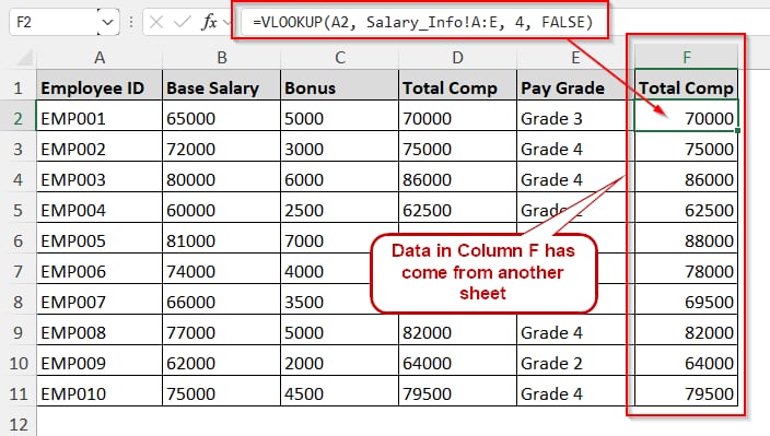
➤ To bring Total Compensation data from another sheet, click F2 on a worksheet and Write Formula on the formula bar. Then Click Enter.
➤ Then drag the fill handle to autofill whole column,
In this article, we’ll look into multiple methods to merge two Excel sheets based on one column. We will use functions like VLOOKUP, XLOOKUP, INDEX MATCH, and tools like Power Query.
Merging Excel Sheets Using the VLOOKUP Formula
The VLOOKUP formula is one of the easiest ways that we use to merge data from two Excel sheets. It is based on a common column: typically an ID or key.
You can use this method when both sheets have a shared identifier, For example: Employee ID, and you want to pull in matching data (like salary or department) from one sheet into another.
Steps:
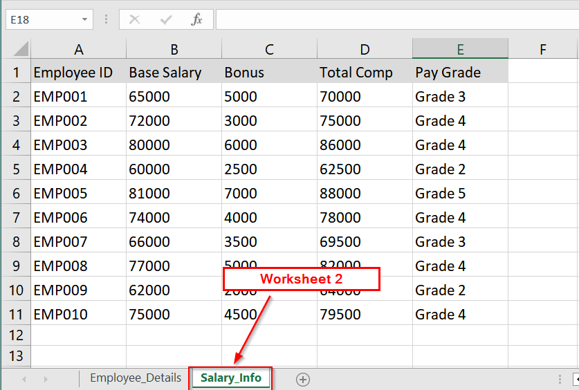
➤ Open Both Excel Sheets where you want to merge data. Make sure that both sheets (e.g., Employee_Details and Salary_Info) are in the same workbook or accessible in separate workbooks.
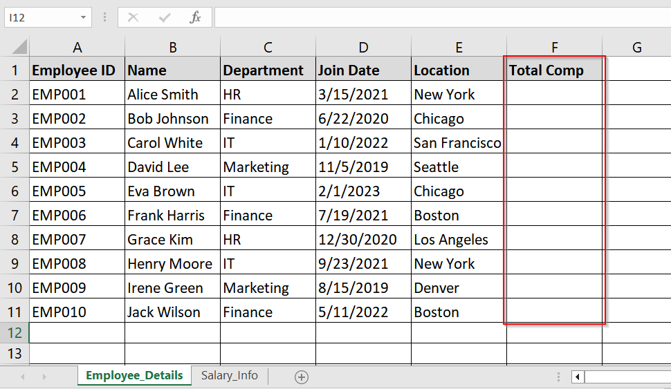
Worksheet 1-

Worksheet 2-
➤ Decide the Destination for the Merged Data. To do that, go to the sheet where you want to pull the information. For example, in Employee_Details, you want to pull Total Comp from Salary_Info.
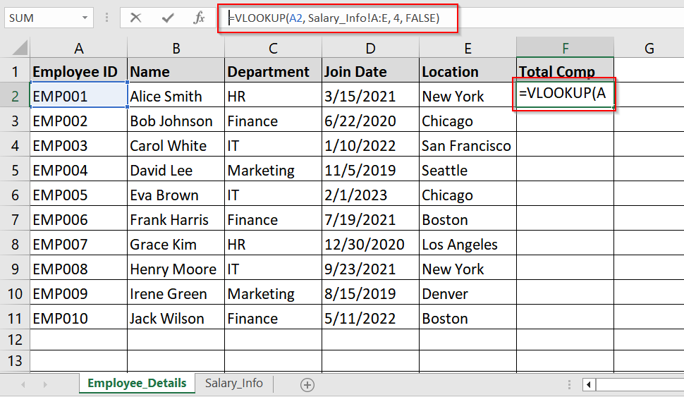
➤ Enter the VLOOKUP Formula in the destination column (Here, F2 Cell)
=VLOOKUP(A2, Salary_Info!A:E, 4, FALSE)
➧ Salary_Info!A:E: The range in the other sheet to search in.
➧ 4: The column index in the range to pull data from (4 = Total Comp).
➧ FALSE: It ensures an exact match.
➤ Copy the Formula Down the Column. To do that, drag the fill handle down the entire column to apply the formula to all rows.
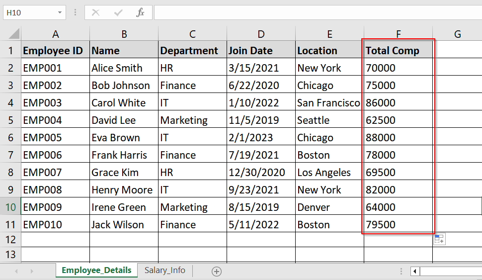
Here’s the final output:

Note:
➧ Make sure that the Employee ID format is consistent in both sheets (e.g., no extra spaces).
➧ VLOOKUP only pulls the first match, and it won’t work if the ID isn’t found in the lookup table.
Using XLOOKUP Function To Merge Excel Sheets
XLOOKUP is a modern and more flexible alternative formula to VLOOKUP in Excel. It allows you to merge two sheets based on a common column without worrying about the lookup column’s position. Use XLOOKUP when you want to match values (like Employee ID) from one sheet and bring related data (like Total Compensation) from another.
Steps:
➤ Open the Excel Sheets and Ensure you have both sheets open-
- Employee_Details
- Salary_Info
These can be in the same workbook or across different files.
➤ Go to Employee_Details and create a new column (e.g., “Total Comp”) next to existing data.

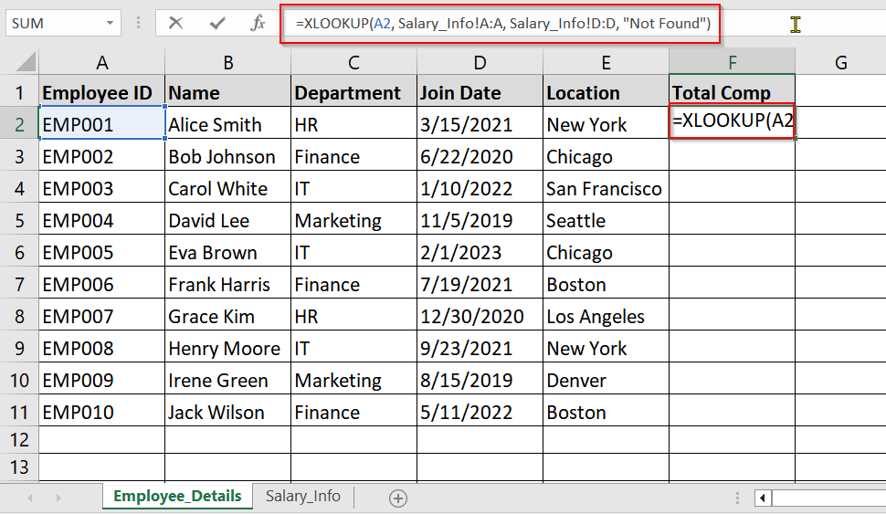
➤ In the first row under the “Total Comp” column, enter:
=XLOOKUP(A2, Salary_Info!A:A, Salary_Info!D:D, “Not Found”)
➤ Use the fill handle to apply the formula to all rows in the column.
➧ XLOOKUP works even if the lookup column is not the first column (unlike VLOOKUP).
➧ XLOOKUP is available in Excel 365 and Excel 2019+. If you’re using an earlier version, it won’t work.
Apply INDEX MATCH Formula To Merge Excel Sheets
The INDEX MATCH formula is a powerful and flexible alternative to VLOOKUP. It’s very useful when your lookup column isn’t the first column. Or when you want better performance with large datasets. In this example, we’ll merge exam scores from one sheet into student information using the Student ID column.
Steps:
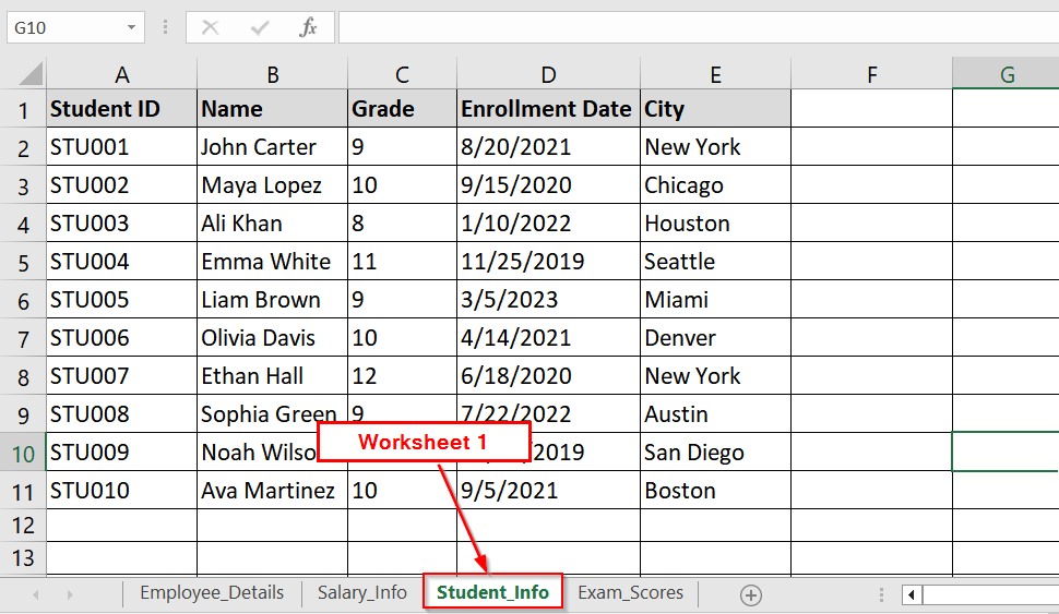
➤ Ensure that both Student_Info and Exam_Scores sheets are available in the same workbook.
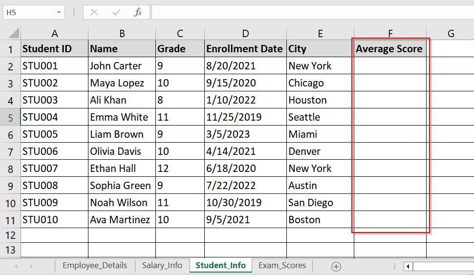
Student_Info Worksheet-
Exam_Scores Worksheet-
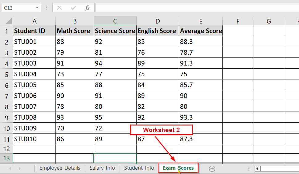
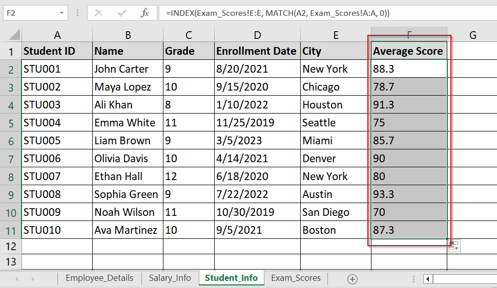
➤ In the Student_Info sheet, insert a new column titled “Average Score” where the data will be pulled in from the Exam_Scores sheet.
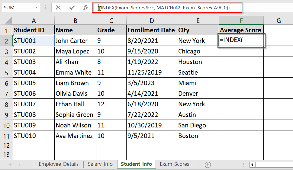
➤ In the first cell of the new “Average Score” column (e.g., cell F2), enter the following formula:
=INDEX(Exam_Scores!E:E, MATCH(A2, Exam_Scores!A:A, 0))
➧ MATCH(A2, Exam_Scores!A:A, 0) then finds the row in Exam_Scores where the Student ID matches the one in cell A2.
➧ 0 indicates an exact match.
➤ Drag the fill handle down the entire “Average Score” column to copy the formula for all students.
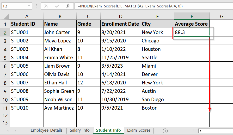
Final View-
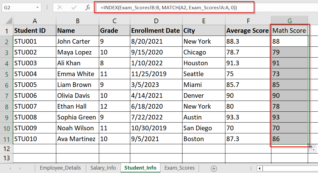
➤ (Optional) Repeat the process to bring in Math, Science, or English scores by changing the column index in INDEX.
Math Score:
=INDEX(Exam_Scores!B:B, MATCH(A2, Exam_Scores!A:A, 0))
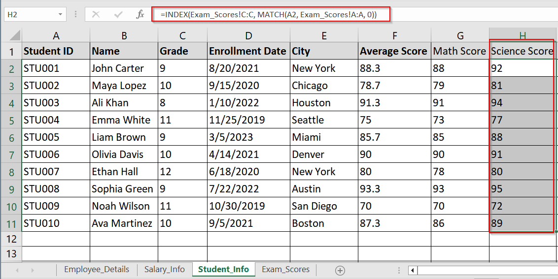
Science Score:
=INDEX(Exam_Scores!C:C, MATCH(A2, Exam_Scores!A:A, 0))
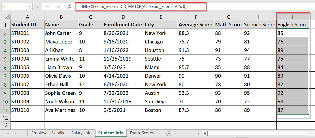
English Score:
=INDEX(Exam_Scores!D:D, MATCH(A2, Exam_Scores!A:A, 0))
➧ INDEX MATCH works left to right or right to left, unlike VLOOKUP.
➧ Always check that Student IDs in both sheets match exactly. You should watch for extra spaces.
➧ Use absolute references (e.g., $A$2:$A$11) if needed to avoid breaking the formula during copying.
Use Power Query To Merge Excel Sheets
Power Query is a data connection and transformation tool. It was built into Excel (Excel 2016 and later). It’s perfect if you are merging large tables by using a common key like Employee ID. You can do it without writing any formulas. This method is good when your datasets are updated frequently, and you want an easy way to refresh your merged data with one click.
Here we will merge:
- Employee_Details → It contains employee info like name and department
- Salary_Info → It contains compensation data like base salary and bonuses
Steps:
➤ Before using Power Query, we have to make the both data ranges formatted as official Excel Tables.
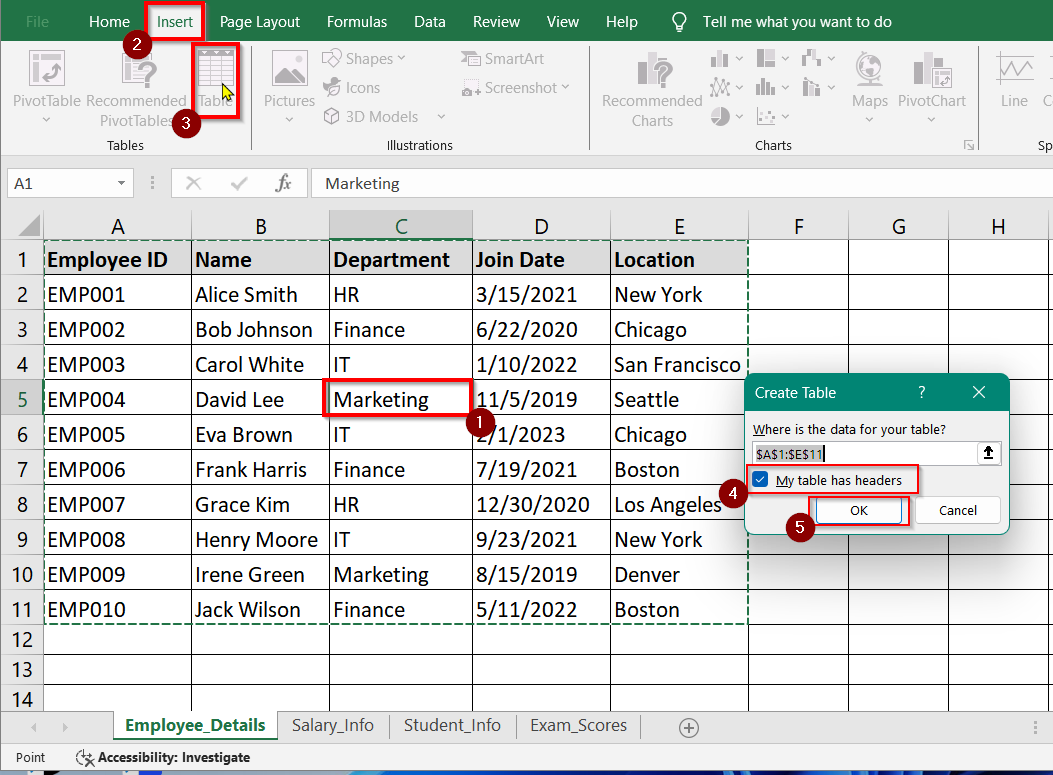
➤ Select any cell in your first dataset (Employee_Details)
➤ Go to Insert tab → click Table
➤ Ensure “My table has headers” is checked → click OK
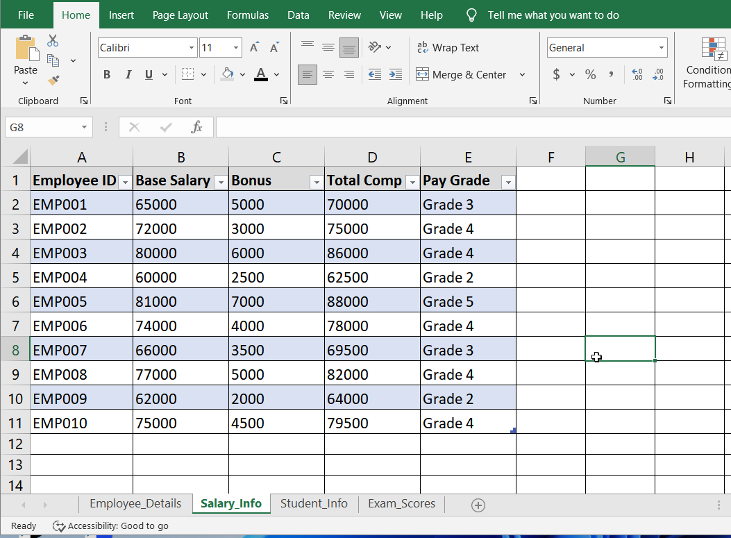
➤ Do the same for the second dataset (Salary_Info) and the result will look like this-
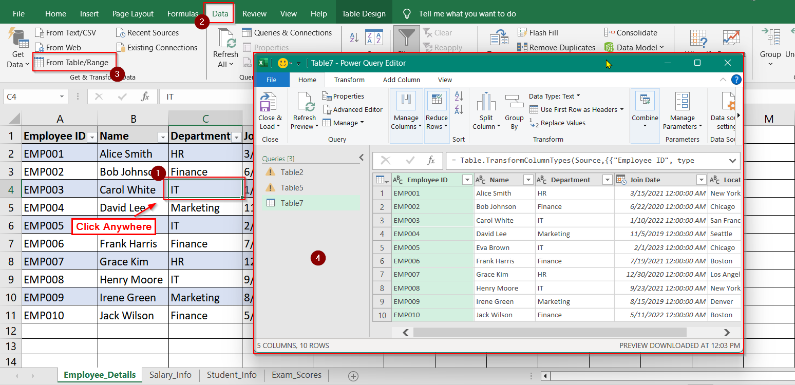
➤ Load the Tables into Power Query by selecting elect any cell in Employee_Details_Table
➤ Go to the Data tab → click From Table/Range under Get & Transform Data. This opens Power Query Editor with the first table
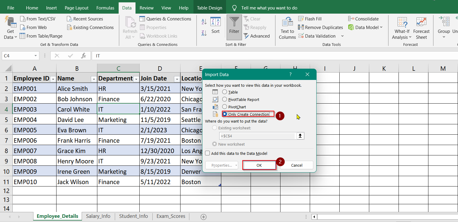
➤ Click Home → Close & Load To…
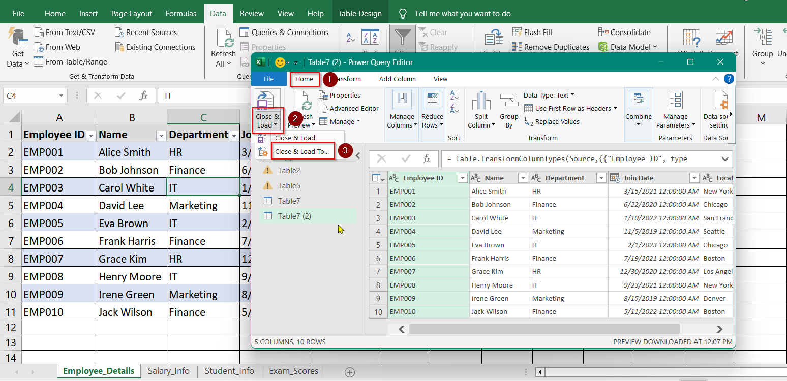
➤ In the new window, choose Only Create Connection-
Repeat the process for Salary_Info Table
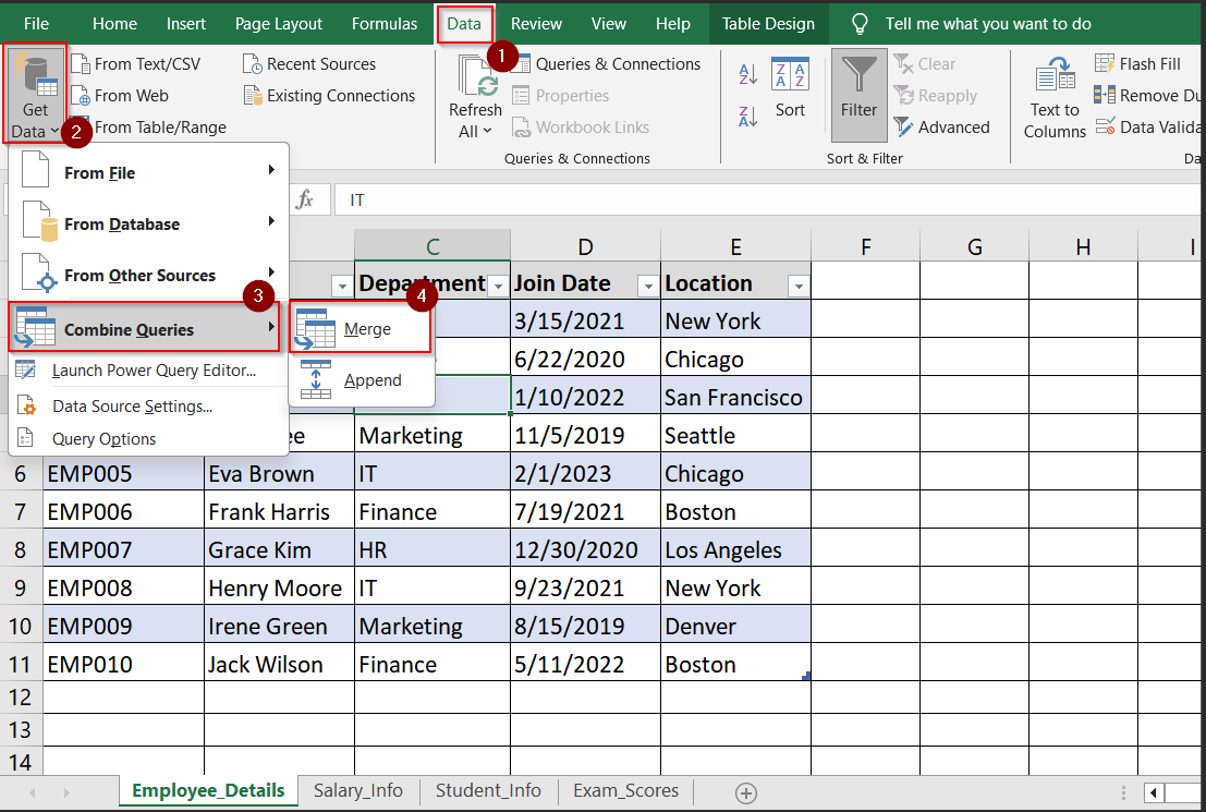
➤ Merge the Two Tables
Go to Data tab → Get Data → Combine Queries → Merge
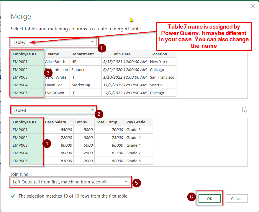
In the Merge dialog:
- First table: select Employee_Details (Here Table 7)
- Second table: select Salary_Info (Here Table 8)
- Select the Employee ID column in both tables
- Join type: choose Left Outer (all from first, matching from second)
Note:
Left Outer Join means you’ll keep all rows from Employee_Details and bring in matching salary info from Salary_Info.
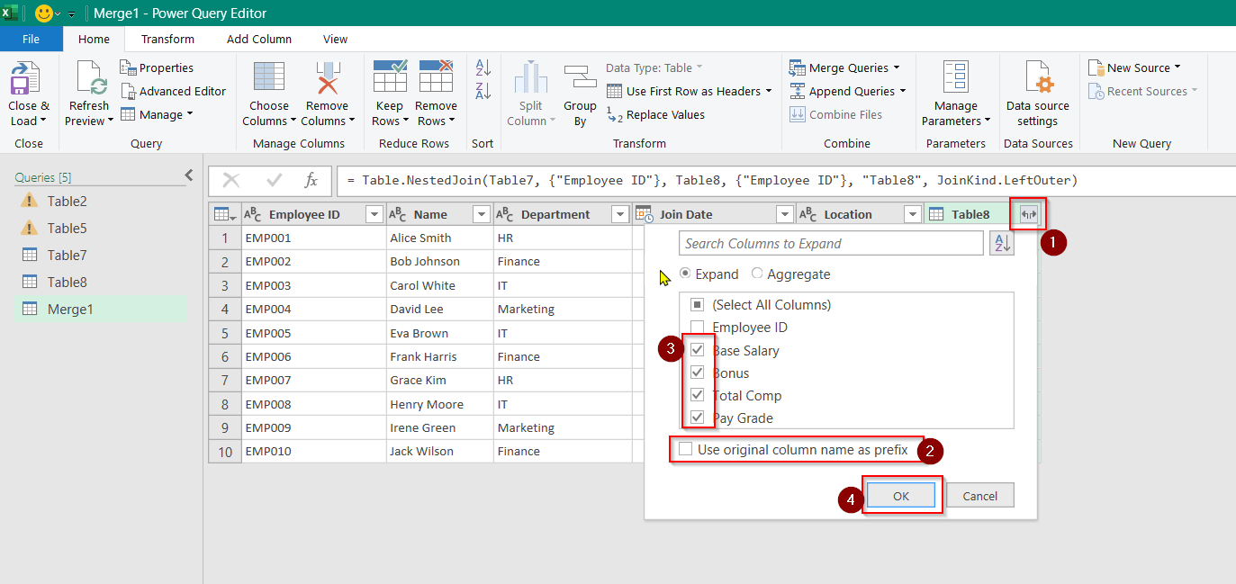
➤ Expand the Merged Table.
➤ After clicking OK, you’ll see a new column named Merge 1.
➤ Click the expand icon (small box with arrow) next to the column header.
➤ In the drop-down:
- Uncheck “Use original column name as prefix”
- Select only the columns you want to bring in (e.g., Base Salary, Bonus, Total Comp, Pay Grade)
- Click OK
➤ Load the Merged Table to Excel
- Click the Home tab in Power Query Editor.
- Then Click Close & Load
- Choose to load it as a new worksheet or table in an existing sheet
You will see a new worksheet like this-
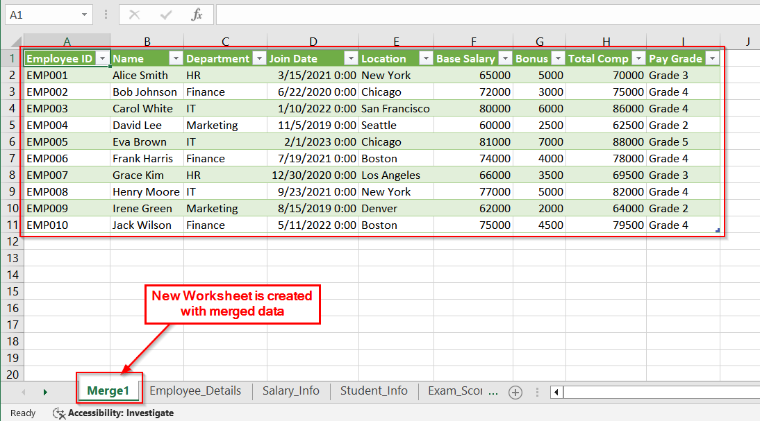
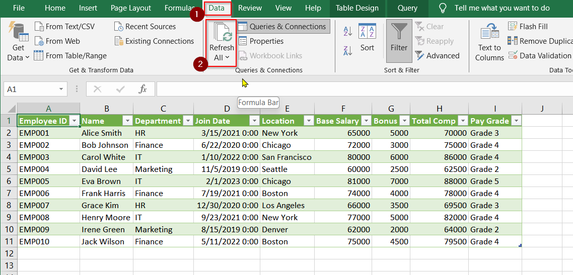
➤ Now that your data is merged using Power Query:
- Anytime your source tables (Employee_Details, Salary_Info) are updated,
- Just click Data tab → Refresh All
The merged data will update without redoing the steps
➧ Power Query creates a snapshot of the data. It does not modify the original tables.
➧ Changes to source data are not live. You must refresh to see updates.
Frequently Asked Questions (FAQs)
How to merge multiple Excel sheets into one?
We can do that by using Power Query to import and combine multiple sheets using “Append” or “Merge” options.
How to merge two column data in one column in Excel?
You can use =A1 & ” ” & B1 or TEXTJOIN to combine data from two columns into one.
How do I automatically link data from one sheet to another in Excel?
You can use formula =Sheet2!A2 to create live links, or use Power Query to establish refreshable connections.
Concluding Words
Knowing how to merge two Excel sheets based on one column is a foundational skill. It can save hours of manual work. We have shown simple formulas like VLOOKUP to advanced tools like Power Query. Choose the method that suits your data structure and Excel version and let Excel do the heavy lifting. Leave a comment below with your valuable feedback.