Merging data from two Excel sheets is a common task for anyone managing lists, sales records, or inventories. One of the easiest and most popular ways to combine information based on a common key or ID is using the VLOOKUP function. It lets you pull matching data from one sheet into another, effectively merging them without manual copying.
In this article, you’ll learn multiple methods to merge two Excel sheets using VLOOKUP function, including variations with other functions like INDIRECT, multi-source lookups using IF, and techniques to handle missing data neatly.
Steps to use VLOOKUP to merge two Excel sheets:
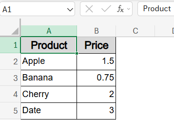
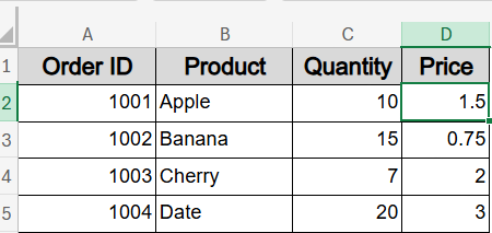
➤ Suppose Sheet2 has two columns called Product and Price ranging from A1:B5.
➤ Go to Sheet1 and select the first blank column next to your data (e.g., D1), name it “Price”.
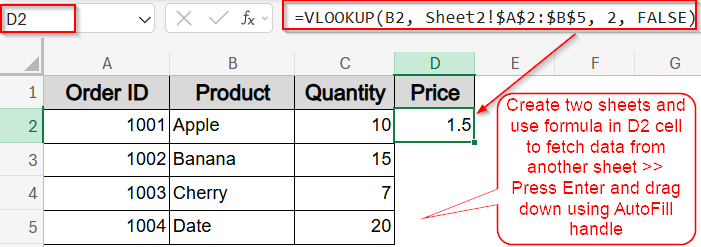
➤ In cell D2, enter this formula:
=VLOOKUP(B2, Sheet2!$A$2:$B$5, 2, FALSE)
Here, B2 is the lookup value (Product in Sheet1), Sheet2!$A$2:$B$5 is the lookup range in Sheet2, 2 means return the value from the 2nd column (Price) and FALSE ensures an exact match.
➤ Press Enter, then drag the formula down to fill all rows.
Standard Merge Using VLOOKUP from Another Sheet
The standard VLOOKUP method is best when you have two sheets with a shared column like “Product” and you want to pull related data such as Price from one sheet into the other.
Steps:
➤ Suppose Sheet2 has two columns called Product and Price ranging from A1:B5.
➤ Go to Sheet1 and select the first blank column next to your data (e.g., D1), name it “Price”.
➤ In cell D2, enter this formula:
Here, B2 is the lookup value (Product in Sheet1), Sheet2!$A$2:$B$5 is the lookup range in Sheet2, 2 means return the value from the 2nd column (Price) and FALSE ensures an exact match.
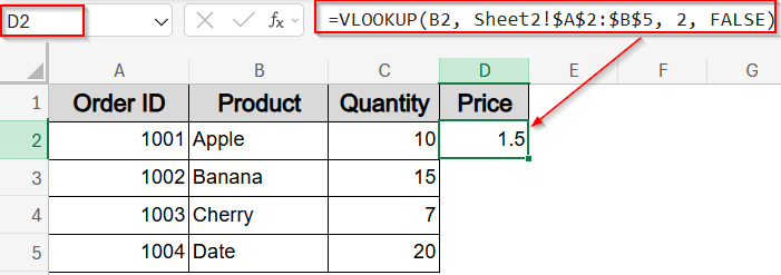
➤ Press Enter, then drag the formula down to fill all rows.
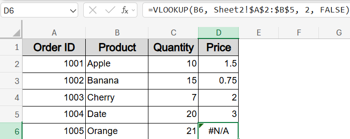
Your Sheet1 now includes the matching prices from Sheet2.
➤ If no match is found, VLOOKUP returns #N/A like in row 6.
➤ To avoid this issue, enter the formula with IFERROR to handle errors neatly in D2 cell:
=IFERROR(VLOOKUP(B2, Sheet2!$A$2:$B$5, 2, FALSE), “Not Found”)
➤ Drag down using the AutoFill handle.
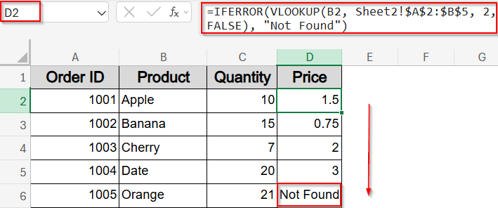
Now your data is neatly presented, even in case of errors.
Dynamic Merge Using Named Range and INDIRECT Function
This method works well if you want a more flexible formula setup, where the lookup range isn’t tied to a specific hardcoded sheet name. It’s helpful for dynamic workbooks with named tables.
Steps:
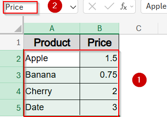
➤ Select range A2:B5 in Sheet2.
➤ Name the range Price by editing inside the Name box next to the Formula Bar.
➤ Go to Sheet1 and insert a new column named Price.
➤ In cell D2, use this formula:
=VLOOKUP(B2, INDIRECT(“Price”), 2, FALSE)
➤ Press Enter and drag down using the AutoFill handle.
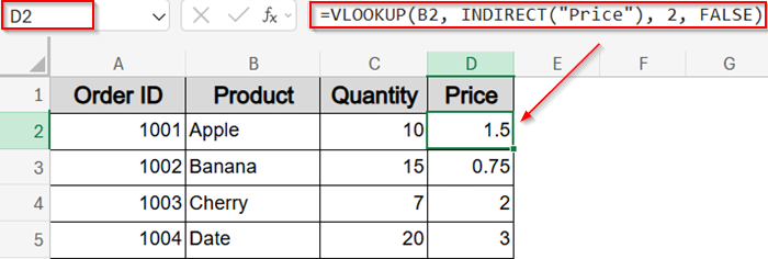
This setup allows dynamic lookup without locking the formula to a specific sheet or cell range.
Conditional Merge from Multiple Sheets Using IF and VLOOKUP Functions
If your pricing is split across multiple sheets based on product categories like Fruit and Dry Fruit, you can use IF function combined with VLOOKUP to decide which sheet to use for each lookup.
Steps:
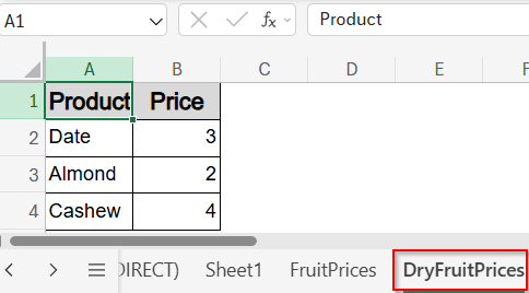
➤ Create a new sheet called FruitPrices and fill it with your suitable data.

➤ Create another sheet called DryFruitPrices in the same way.
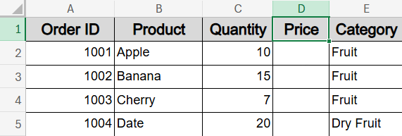
➤ Go to Sheet1, and insert a new column named Price in column D and Category in Column E. Fill column E with category names such as Fruit and Dry Fruit.
➤ In cell D2, enter the following formula:
=IF(E2=”Fruit”, VLOOKUP(B2, FruitPrices!$A$2:$B$100, 2, FALSE), IF(E2=”Dry Fruit”, VLOOKUP(B2, DryFruitPrices!$A$2:$B$100, 2, FALSE),“Not Found”))
➤ Press Enter and drag down using the AutoFill handle.
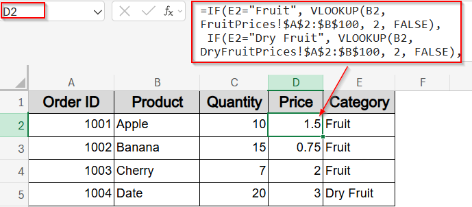
Your sheet will now display the correct price for each product based on its assigned category and lookup sheet creating a dynamic category-driven pricing merge.
Frequently Asked Questions
Can I use VLOOKUP with three or more sheets?
Yes, you can use IFERROR or nested IF statements to check multiple sheets one after another. This allows Excel to search in each sheet until a match is found.
What if I want to return multiple columns of data, not just one?
VLOOKUP function only returns one column at a time. To fetch multiple values, combine multiple VLOOKUPs in adjacent columns, or use INDEX-MATCH with structured arrays for better control and flexibility.
How do I handle case mismatches like “apple” vs “Apple”?
By default, VLOOKUP ignores case sensitivity. To perform case-sensitive lookups, use a formula combining INDEX, MATCH, and EXACT, which ensures an exact match considering letter case differences.
Is VLOOKUP better than XLOOKUP?
XLOOKUP is more versatile than VLOOKUP since it allows searching in any direction, supports default error values, and handles arrays better. But VLOOKUP is still reliable and works in older Excel versions.
Wrapping Up
In this tutorial, you learned how to use the VLOOKUP function to merge two Excel sheets using multiple techniques, from simple lookups to category-driven logic using multiple sheets. Whether you’re pulling in prices, names, IDs, or other related data, VLOOKUP function makes merging structured and efficient. Feel free to download the practice file and share your feedback.